You will need your calculator today and every

You will need your calculator today (and every day from now on)

Chapter 2 Descriptive Statistics

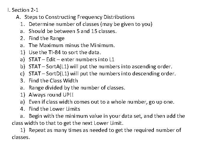
I. Section 2 -1 A. Steps to Constructing Frequency Distributions 1. Determine number of classes (may be given to you) a. Should be between 5 and 15 classes. 2. Find the Range a. The Maximum minus the Minimum. 1) Use the TI-84 to sort the data. a) STAT – Edit – enter numbers into L 1 b) STAT – Sort. A(L 1) will put the numbers into ascending order. c) STAT – Sort. D(L 1) will put the numbers into descending order. 3. Find the Class Width a. Range divided by the number of classes. 1) Always round UP!! a) Even if class width comes out to a whole number, go up one. 4. Find the Lower Limits a. Begin with the minimum value in your data set, and then add the class width to that to get the next Lower Limit. 1) Repeat as many times as needed to get the required number of classes.

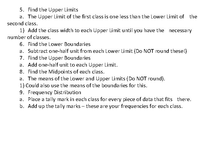
5. Find the Upper Limits a. The Upper Limit of the first class is one less than the Lower Limit of the second class. 1) Add the class width to each Upper Limit until you have the necessary number of classes. 6. Find the Lower Boundaries a. Subtract one-half unit from each Lower Limit (Do NOT round these!) 7. Find the Upper Boundaries a. Add one-half unit to each Upper Limit. 8. Find the Midpoints of each class. a. The means of the Lower and Upper Limits (Do NOT round). 1) Could also use the means of the boundaries for this. 9. Frequency Distribution a. Place a tally mark in each class for every piece of data that fits there. b. Add up the tally marks – these are your frequencies for each class.

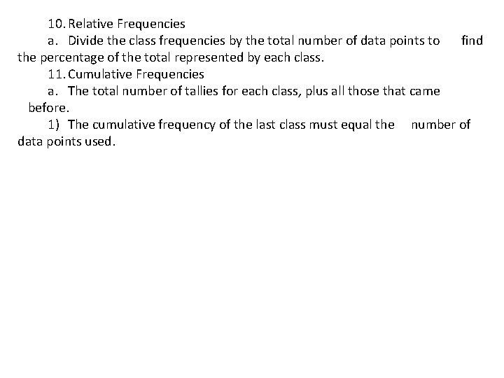
10. Relative Frequencies a. Divide the class frequencies by the total number of data points to find the percentage of the total represented by each class. 11. Cumulative Frequencies a. The total number of tallies for each class, plus all those that came before. 1) The cumulative frequency of the last class must equal the number of data points used.

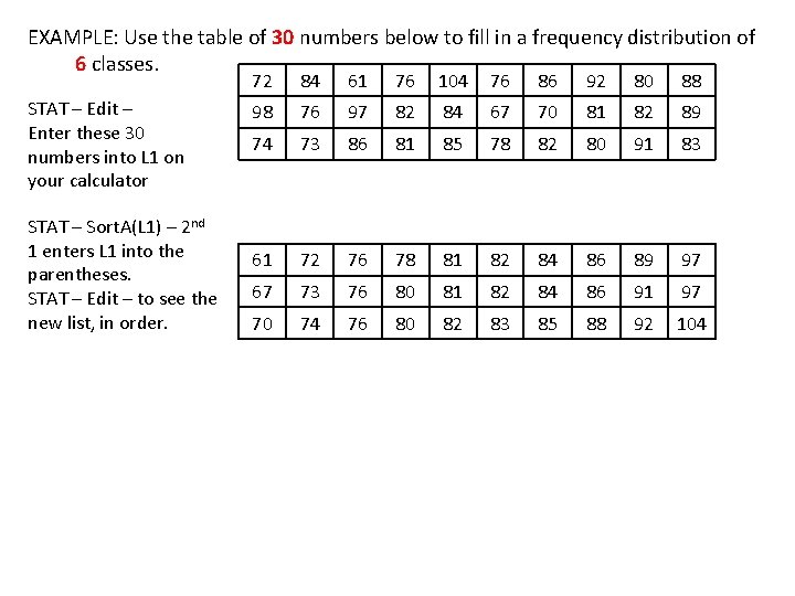
EXAMPLE: Use the table of 30 numbers below to fill in a frequency distribution of 6 classes. STAT – Edit – Enter these 30 numbers into L 1 on your calculator STAT – Sort. A(L 1) – 2 nd 1 enters L 1 into the parentheses. STAT – Edit – to see the new list, in order. 72 84 61 76 104 76 86 92 80 88 98 76 97 82 84 67 70 81 82 89 74 73 86 81 85 78 82 80 91 83 61 72 76 78 81 82 84 86 89 97 67 73 76 80 81 82 84 86 91 97 70 74 76 80 82 83 85 88 92 104

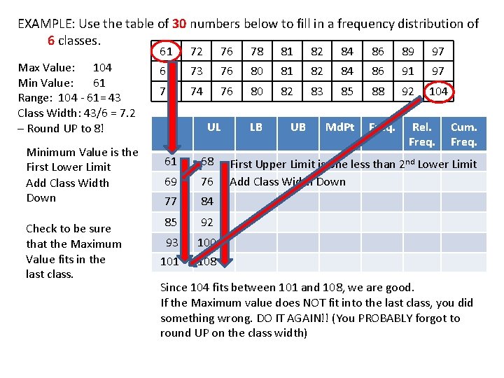
EXAMPLE: Use the table of 30 numbers below to fill in a frequency distribution of 6 classes. Max Value: 104 Min Value: 61 Range: 104 - 61= 43 Class Width: 43/6 = 7. 2 – Round UP to 8! Minimum Value is the First Lower Limit Add Class Width Down Check to be sure that the Maximum Value fits in the last class. 61 72 76 78 81 82 84 86 89 97 67 73 76 80 81 82 84 86 91 97 70 74 76 80 82 83 85 88 92 104 LL UL 61 68 69 76 77 84 85 92 93 100 101 108 LB UB Md. Pt Freq. Rel. Freq. Cum. Freq. First Upper Limit is one less than 2 nd Lower Limit Add Class Width Down Since 104 fits between 101 and 108, we are good. If the Maximum value does NOT fit into the last class, you did something wrong. DO IT AGAIN!! (You PROBABLY forgot to round UP on the class width)

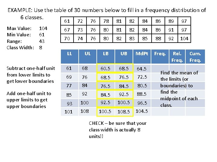
EXAMPLE: Use the table of 30 numbers below to fill in a frequency distribution of 6 classes. Max Value: Min Value: Range: Class Width: 104 61 43 8 61 72 76 78 81 82 84 86 89 97 67 73 76 80 81 82 84 86 91 97 70 74 76 80 82 83 85 88 92 104 LL UL LB UB Md. Pt Subtract one-half unit from lower limits to get lower boundaries 61 68 60. 5 68. 5 69 76 68. 5 76. 5 64. 5 72. 5 77 84 76. 5 84. 5 80. 5 Add one-half unit to upper limits to get upper boundaries 85 92 92. 5 88. 5 93 101 100 84. 5 92. 5 100. 5 108. 5 96. 5 104. 5 CHECK – be sure that your class width is actually 8 units!! Freq. Rel. Freq. Cum. Freq. Find the mean of the limits (or boundaries) to find the midpoint of each class.

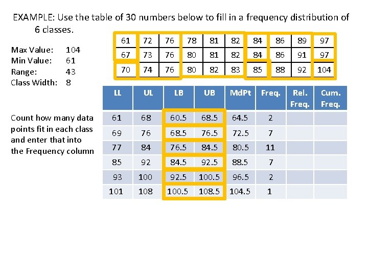
EXAMPLE: Use the table of 30 numbers below to fill in a frequency distribution of 6 classes. Max Value: Min Value: Range: Class Width: 104 61 43 8 Count how many data points fit in each class and enter that into the Frequency column 61 72 76 78 81 82 84 86 89 97 67 73 76 80 81 82 84 86 91 97 70 74 76 80 82 83 85 88 92 104 LL UL LB UB Md. Pt Freq. 61 68 60. 5 68. 5 64. 5 2 69 76 68. 5 76. 5 72. 5 7 77 84 76. 5 84. 5 80. 5 11 85 92 84. 5 92. 5 88. 5 7 93 100 92. 5 100. 5 96. 5 2 101 108 100. 5 108. 5 104. 5 1 Rel. Freq. Cum. Freq.

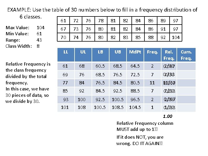
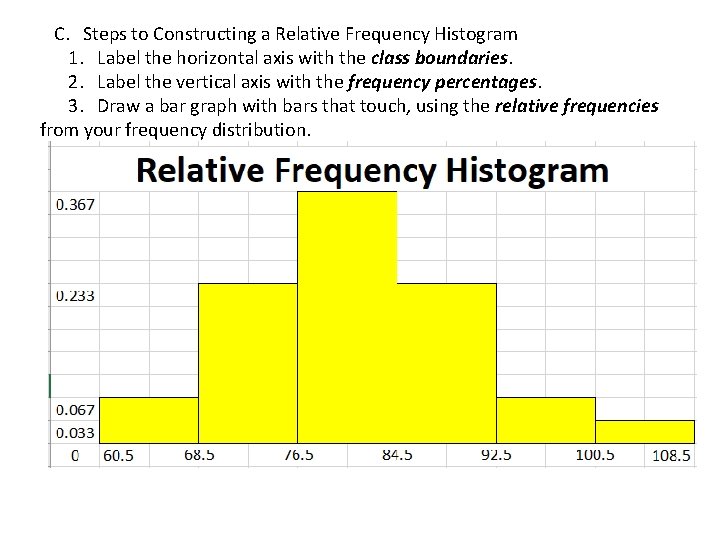
EXAMPLE: Use the table of 30 numbers below to fill in a frequency distribution of 6 classes. Max Value: Min Value: Range: Class Width: 104 61 43 8 Relative Frequency is the class frequency divided by the total frequency. In this case, we have 30 pieces of data, so we divide by 30. 61 72 76 78 81 82 84 86 89 97 67 73 76 80 81 82 84 86 91 97 70 74 76 80 82 83 85 88 92 104 LL UL LB UB Md. Pt Freq. Rel. Freq. 61 68 60. 5 68. 5 64. 5 2 2/30 0. 067 69 76 68. 5 76. 5 72. 5 7 0. 233 7/30 77 84 76. 5 84. 5 80. 5 11 11/30 0. 367 85 92 84. 5 92. 5 88. 5 7 7/30 0. 233 93 100 92. 5 100. 5 96. 5 2 0. 067 2/30 101 108 100. 5 108. 5 104. 5 1 1/30 0. 033 1. 00 Relative Frequency column MUST add up to 1!! If it does NOT, you are wrong. DO IT AGAIN!! Cum. Freq.

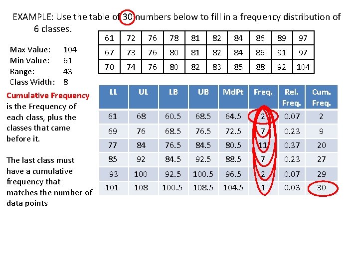
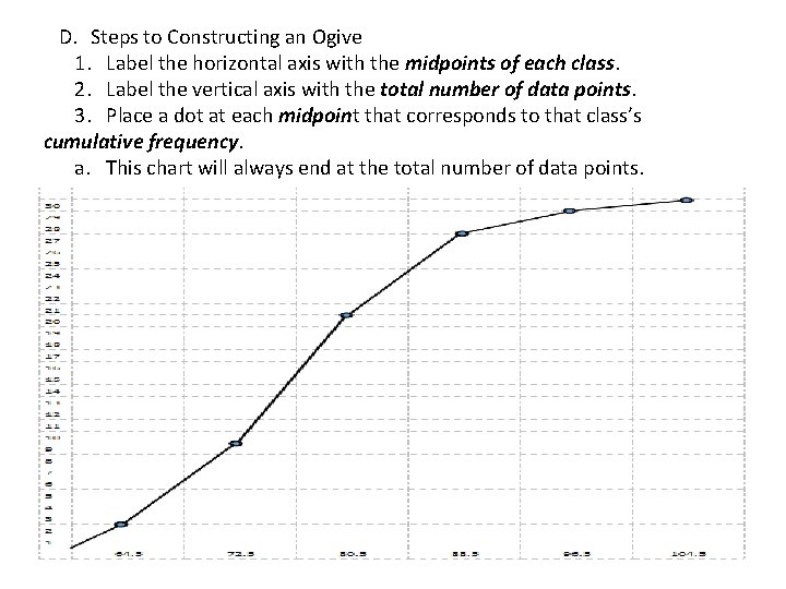
EXAMPLE: Use the table of 30 numbers below to fill in a frequency distribution of 6 classes. Max Value: Min Value: Range: Class Width: 104 61 43 8 Cumulative Frequency is the Frequency of each class, plus the classes that came before it. The last class must have a cumulative frequency that matches the number of data points 61 72 76 78 81 82 84 86 89 97 67 73 76 80 81 82 84 86 91 97 70 74 76 80 82 83 85 88 92 104 LL UL LB UB Md. Pt Freq. Rel. Freq. Cum. Freq. 61 68 60. 5 68. 5 64. 5 2 0. 07 2 69 76 68. 5 76. 5 72. 5 7 0. 23 9 77 84 76. 5 84. 5 80. 5 11 0. 37 20 85 92 84. 5 92. 5 88. 5 7 0. 23 27 93 100 92. 5 100. 5 96. 5 2 0. 07 29 101 108 100. 5 108. 5 104. 5 1 0. 03 30

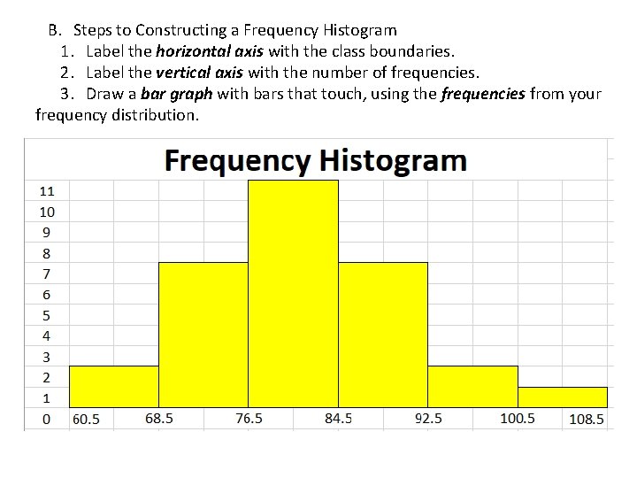
B. Steps to Constructing a Frequency Histogram 1. Label the horizontal axis with the class boundaries. 2. Label the vertical axis with the number of frequencies. 3. Draw a bar graph with bars that touch, using the frequencies from your frequency distribution.

C. Steps to Constructing a Relative Frequency Histogram 1. Label the horizontal axis with the class boundaries. 2. Label the vertical axis with the frequency percentages. 3. Draw a bar graph with bars that touch, using the relative frequencies from your frequency distribution.

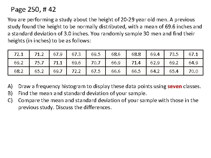
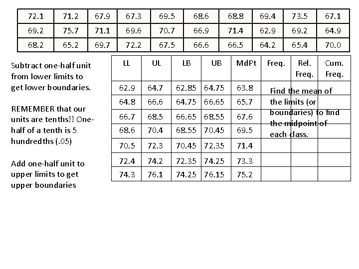
Page 250, # 42 You are performing a study about the height of 20 -29 year old men. A previous study found the height to be normally distributed, with a mean of 69. 6 inches and a standard deviation of 3. 0 inches. You randomly sample 30 men and find their heights (in inches) to be as follows: 72. 1 71. 2 67. 9 67. 3 69. 5 68. 6 68. 8 69. 4 73. 5 67. 1 69. 2 75. 7 71. 1 69. 6 70. 7 66. 9 71. 4 62. 9 69. 2 64. 9 68. 2 65. 2 69. 7 72. 2 67. 5 66. 6 66. 5 64. 2 65. 4 70. 0 A) Draw a frequency histogram to display these data points using seven classes. B) Find the mean and standard deviation of your sample. C) Compare the mean and standard deviation of your sample with those in the previous study. Discuss the differences.

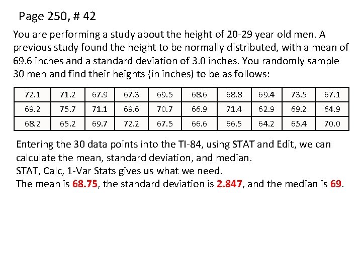
Page 250, # 42 You are performing a study about the height of 20 -29 year old men. A previous study found the height to be normally distributed, with a mean of 69. 6 inches and a standard deviation of 3. 0 inches. You randomly sample 30 men and find their heights (in inches) to be as follows: 72. 1 71. 2 67. 9 67. 3 69. 5 68. 6 68. 8 69. 4 73. 5 67. 1 69. 2 75. 7 71. 1 69. 6 70. 7 66. 9 71. 4 62. 9 69. 2 64. 9 68. 2 65. 2 69. 7 72. 2 67. 5 66. 6 66. 5 64. 2 65. 4 70. 0 Entering the 30 data points into the TI-84, using STAT and Edit, we can calculate the mean, standard deviation, and median. STAT, Calc, 1 -Var Stats gives us what we need. The mean is 68. 75, the standard deviation is 2. 847, and the median is 69.

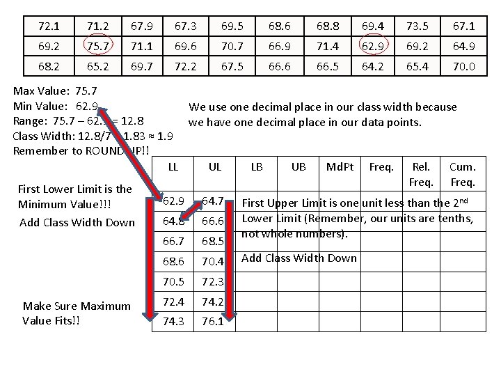
72. 1 71. 2 67. 9 67. 3 69. 5 68. 6 68. 8 69. 4 73. 5 67. 1 69. 2 75. 7 71. 1 69. 6 70. 7 66. 9 71. 4 62. 9 69. 2 64. 9 68. 2 65. 2 69. 7 72. 2 67. 5 66. 6 66. 5 64. 2 65. 4 70. 0 Max Value: 75. 7 Min Value: 62. 9 We use one decimal place in our class width because Range: 75. 7 – 62. 9 = 12. 8 we have one decimal place in our data points. Class Width: 12. 8/7 = 1. 83 ≈ 1. 9 Remember to ROUND UP!! LL UL LB UB Md. Pt Freq. Rel. Cum. Freq. First Lower Limit is the 62. 9 64. 7 First Upper Limit is one unit less than the 2 nd Minimum Value!!! 64. 8 66. 6 Lower Limit (Remember, our units are tenths, Add Class Width Down not whole numbers). 66. 7 68. 5 68. 6 70. 4 Add Class Width Down Make Sure Maximum Value Fits!! 70. 5 72. 3 72. 4 74. 2 74. 3 76. 1

72. 1 71. 2 67. 9 67. 3 69. 5 68. 6 68. 8 69. 4 73. 5 67. 1 69. 2 75. 7 71. 1 69. 6 70. 7 66. 9 71. 4 62. 9 69. 2 64. 9 68. 2 65. 2 69. 7 72. 2 67. 5 66. 6 66. 5 64. 2 65. 4 70. 0 Subtract one-half unit from lower limits to get lower boundaries. REMEMBER that our units are tenths!! Onehalf of a tenth is 5 hundredths (. 05) Add one-half unit to upper limits to get upper boundaries LL UL LB UB Md. Pt 62. 9 64. 7 62. 85 64. 75 63. 8 64. 8 66. 6 64. 75 66. 65 65. 7 66. 7 68. 5 66. 65 68. 55 67. 6 68. 6 70. 4 68. 55 70. 45 69. 5 70. 5 72. 3 70. 45 72. 35 71. 4 72. 4 74. 3 74. 2 76. 1 72. 35 74. 25 76. 15 73. 3 75. 2 Freq. Rel. Freq. Cum. Freq. Find the mean of the limits (or boundaries) to find the midpoint of each class.

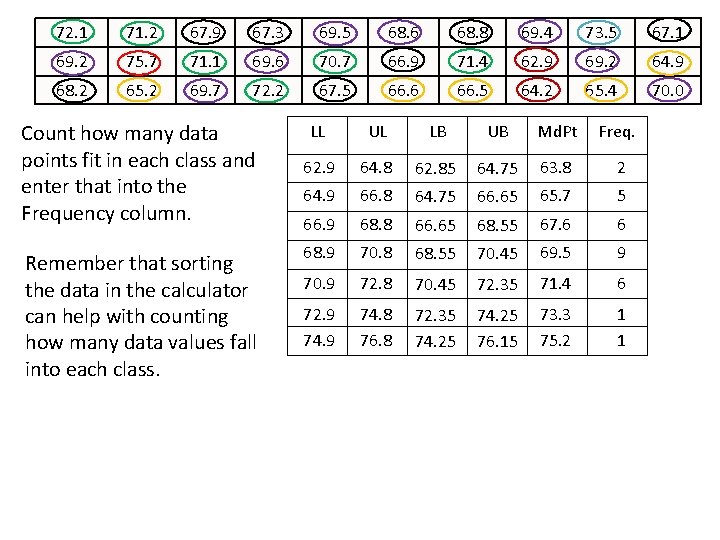
72. 1 71. 2 67. 9 67. 3 69. 5 68. 6 68. 8 69. 4 73. 5 67. 1 69. 2 75. 7 71. 1 69. 6 70. 7 66. 9 71. 4 62. 9 69. 2 64. 9 68. 2 65. 2 69. 7 72. 2 67. 5 66. 6 66. 5 64. 2 65. 4 70. 0 Count how many data points fit in each class and enter that into the Frequency column. Remember that sorting the data in the calculator can help with counting how many data values fall into each class. LL UL LB UB Md. Pt Freq. 62. 9 64. 8 62. 85 64. 75 63. 8 2 64. 9 66. 8 64. 75 66. 65 65. 7 5 66. 9 68. 8 66. 65 68. 55 67. 6 6 68. 9 70. 8 68. 55 70. 45 69. 5 9 70. 9 72. 8 70. 45 72. 35 71. 4 6 72. 9 74. 8 76. 8 72. 35 74. 25 76. 15 73. 3 75. 2 1 1

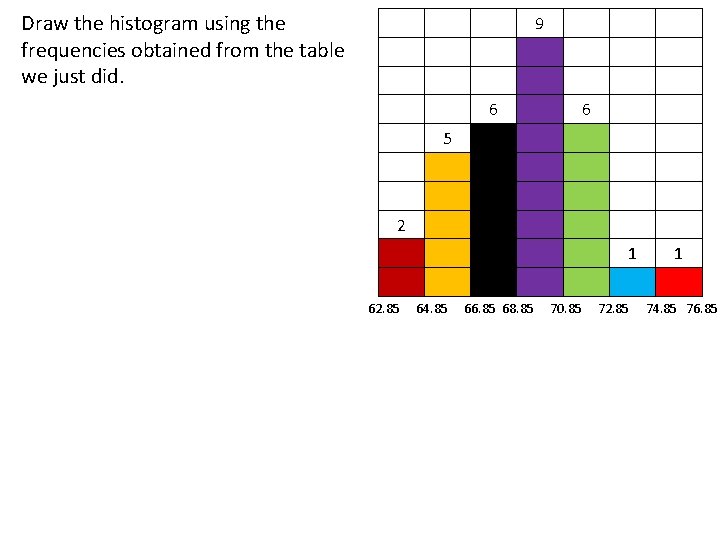
Draw the histogram using the frequencies obtained from the table we just did. 9 6 6 5 2 1 62. 85 64. 85 66. 85 68. 85 70. 85 72. 85 1 74. 85 76. 85

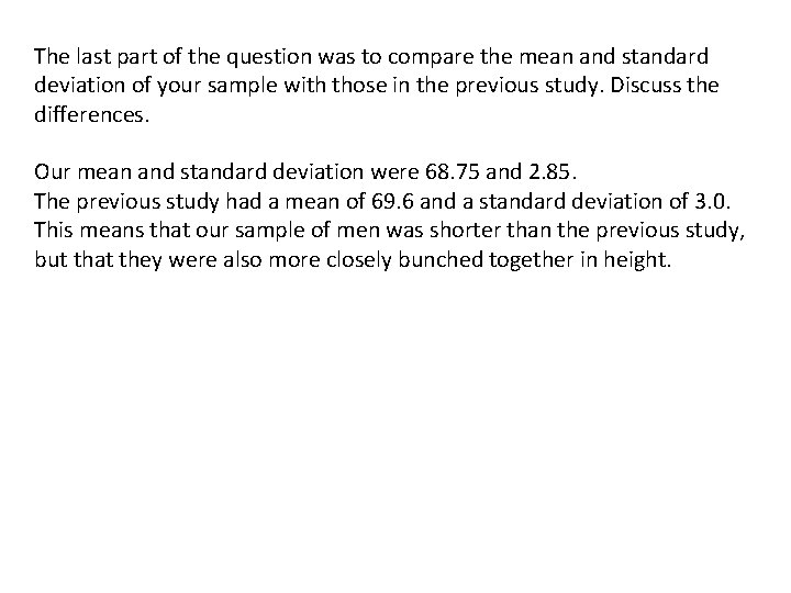
The last part of the question was to compare the mean and standard deviation of your sample with those in the previous study. Discuss the differences. Our mean and standard deviation were 68. 75 and 2. 85. The previous study had a mean of 69. 6 and a standard deviation of 3. 0. This means that our sample of men was shorter than the previous study, but that they were also more closely bunched together in height.

D. Steps to Constructing an Ogive 1. Label the horizontal axis with the midpoints of each class. 2. Label the vertical axis with the total number of data points. 3. Place a dot at each midpoint that corresponds to that class’s cumulative frequency. a. This chart will always end at the total number of data points.

Assignments: Classwork: Pages 49 -51 #1 -8 All, 10 -26 Evens Homework: Pages 52 -53 #29 -41 Odds