YIELD SPREADS Yn Yr I P where Yn

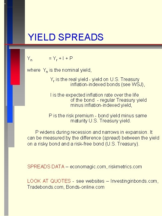
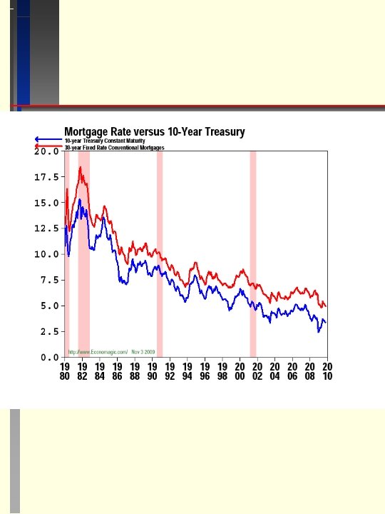
YIELD SPREADS Yn = Yr + I + P where Yn is the nominal yield, Yr is the real yield - yield on U. S. Treasury inflation-indexed bonds (see WSJ), I is the expected inflation rate over the life of the bond - regular Treasury yield minus inflation-indexed yield, P is the risk premium - bond yield minus same maturity U. S. Treasury yield. P widens during recession and narrows in expansion. It can be measured by the difference (spread) between the yield on a risky bond a risk-free bond (U. S. Treasury). SPREADS DATA – economagic. com, riskmetrics. com LOOK AT QUOTES - see websites – Investinginbonds. com, Tradebonds. com, Bonds-online. com

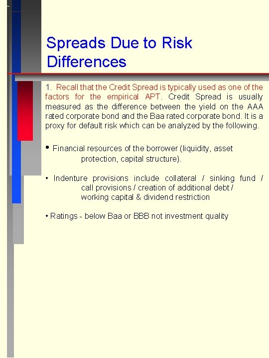
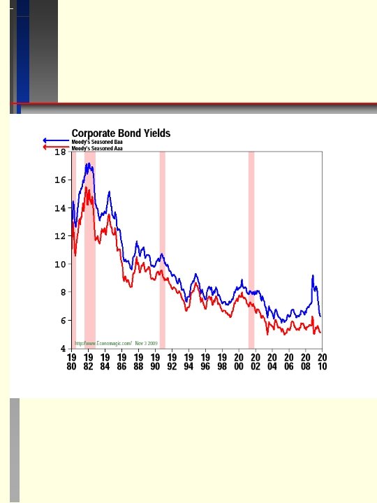
Spreads Due to Risk Differences 1. Recall that the Credit Spread is typically used as one of the factors for the empirical APT. Credit Spread is usually measured as the difference between the yield on the AAA rated corporate bond and the Baa rated corporate bond. It is a proxy for default risk which can be analyzed by the following. • Financial resources of the borrower (liquidity, asset protection, capital structure). • Indenture provisions include collateral / sinking fund / call provisions / creation of additional debt / working capital & dividend restriction • Ratings - below Baa or BBB not investment quality

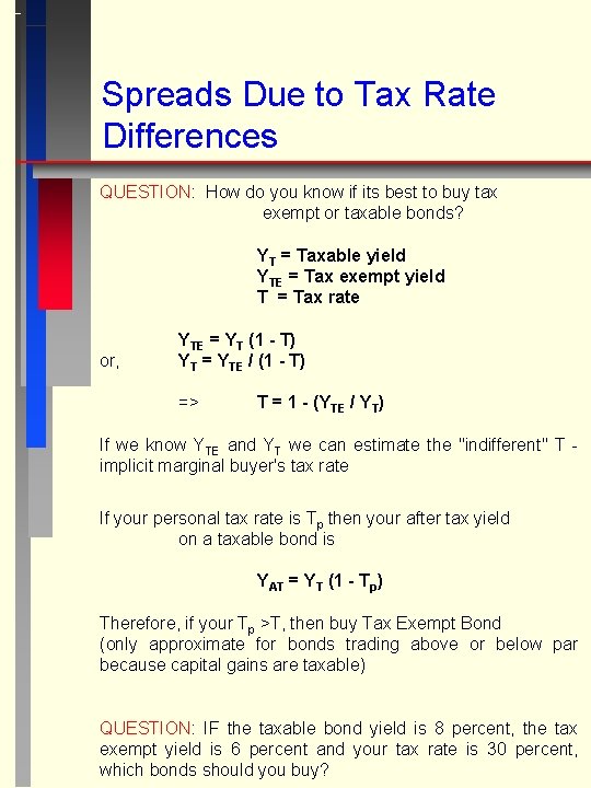
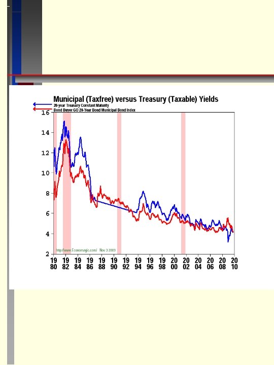
Spreads Due to Tax Rate Differences QUESTION: How do you know if its best to buy tax exempt or taxable bonds? YT = Taxable yield YTE = Tax exempt yield T = Tax rate or, YTE = YT (1 - T) YT = YTE / (1 - T) => T = 1 - (YTE / YT) If we know YTE and YT we can estimate the "indifferent" T implicit marginal buyer's tax rate If your personal tax rate is Tp then your after tax yield on a taxable bond is YAT = YT (1 - Tp) Therefore, if your Tp >T, then buy Tax Exempt Bond (only approximate for bonds trading above or below par because capital gains are taxable) QUESTION: IF the taxable bond yield is 8 percent, the tax exempt yield is 6 percent and your tax rate is 30 percent, which bonds should you buy?

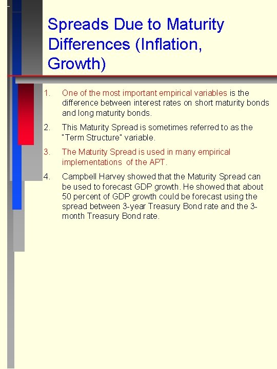
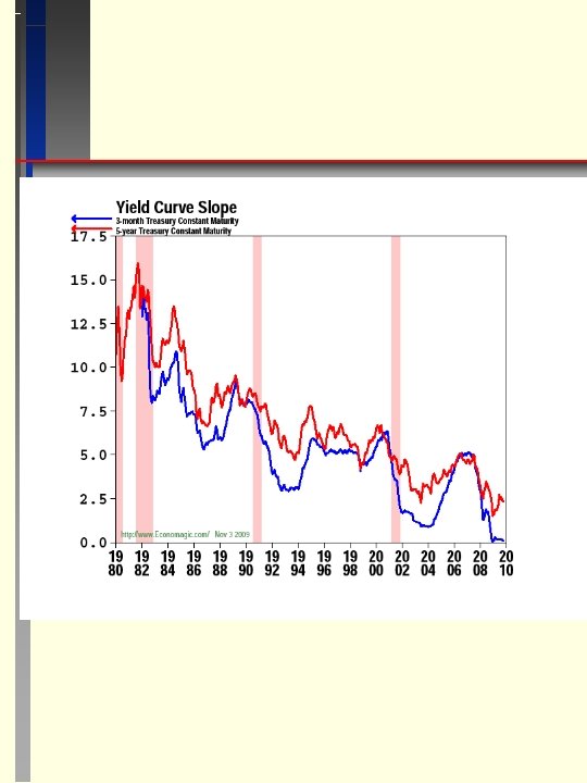
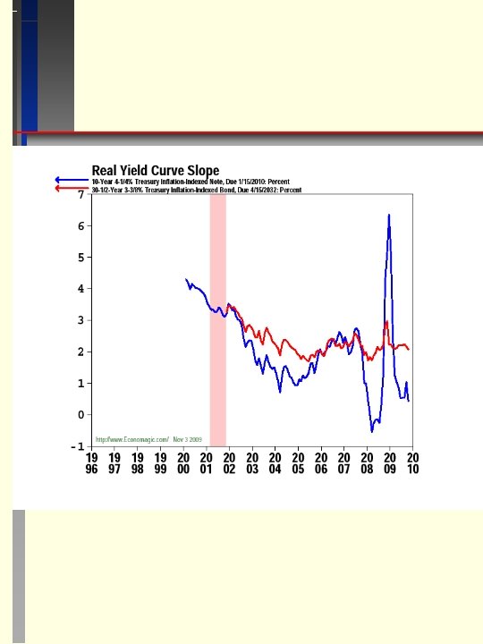
Spreads Due to Maturity Differences (Inflation, Growth) 1. One of the most important empirical variables is the difference between interest rates on short maturity bonds and long maturity bonds. 2. This Maturity Spread is sometimes referred to as the “Term Structure” variable. 3. The Maturity Spread is used in many empirical implementations of the APT. 4. Campbell Harvey showed that the Maturity Spread can be used to forecast GDP growth. He showed that about 50 percent of GDP growth could be forecast using the spread between 3 -year Treasury Bond rate and the 3 month Treasury Bond rate.

5. Harvey showed that the Maturity Spread forecast the last 5 recessions, 4 -5 quarters before the recessions actually started and also predicted when they would end. 6. When the “Yield Curve” inverted significantly (short rate > long rate), recession followed. When the curve changed to flat or normal, then growth in GDP resumed. The size of the inversion (spread) helped predict the severity of the recession as well. (Theoretically, the spread should be between real interest rates although nominal rates are typically used). 7. Harvey shows that this works for many countries besides the U. S. Also, differences in spreads between other countries and the U. S. spread adds additional predictive power beyond a country’s own spread forecasting its GDP. 7. This relationship between Maturity Spread and GDP growth can be explained in two ways. a. When people expect a recession (bad times), they attempt to lock in safe returns for the long term by buying long-term bonds and selling short-term bonds to finance their purchases. This puts pressure on short rates to rise and long rates to fall. b. When businesses expect a recession, they cut back on the more uncertain long-range project and fund short term projects or try to maintain operations in the face of losses. This pressures short rates up and long rates down.

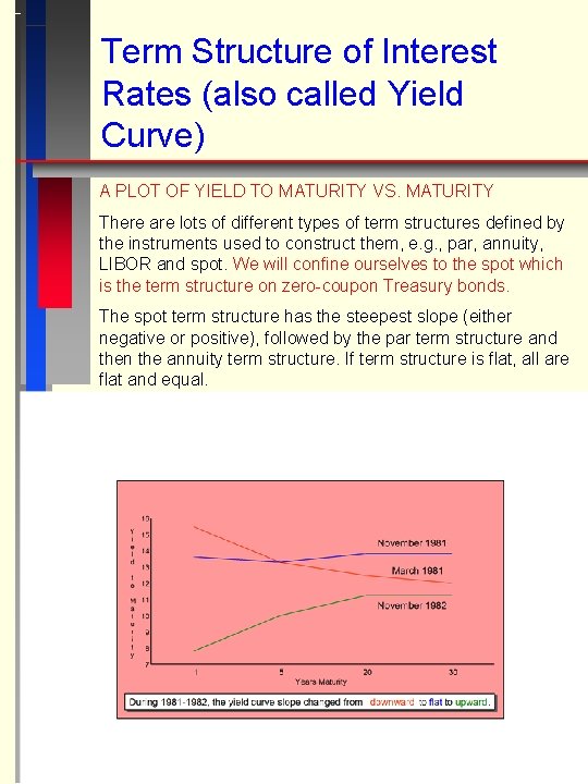
Term Structure of Interest Rates (also called Yield Curve) A PLOT OF YIELD TO MATURITY VS. MATURITY There are lots of different types of term structures defined by the instruments used to construct them, e. g. , par, annuity, LIBOR and spot. We will confine ourselves to the spot which is the term structure on zero-coupon Treasury bonds. The spot term structure has the steepest slope (either negative or positive), followed by the par term structure and then the annuity term structure. If term structure is flat, all are flat and equal.

EXPECTATIONS THEORY OF TERM STRUCTURE 1. The theory assumes that 2. A. Investor’s expectation of future one-period rates are unbiased. B. Different maturity bonds are perfect substitutes 3. Yn = the nominal bond yield for a bond covering n years rn = the expected "forward" yield for a one year bond covering the one year period n. NOTE: r 2 is not the two year bond rate, it is the rate expected on the one year bond next year. (1 + Yn)n = (1 + r 1)(1 + r 2). . . (1 + rn) (1 + Yn) = [(1 + r 1)(1 + r 2). . . (1 + rn)]1/n This implies that any nominal long bond yield can be expressed as a geometric average of one year rates. QUESTION: Why must this hold? ANSWER: Because you always have the option of holding one year bonds and rolling them over. If this were not true then one could arbitrage. Look At Living Yield Curve – Smartmoney. com

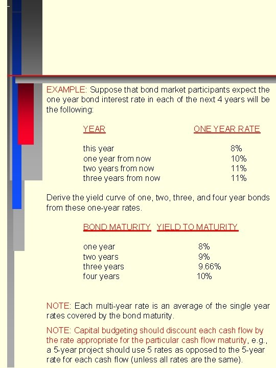
EXAMPLE: Suppose that bond market participants expect the one year bond interest rate in each of the next 4 years will be the following: YEAR ONE YEAR RATE this year one year from now two years from now three years from now 8% 10% 11% Derive the yield curve of one, two, three, and four year bonds from these one-year rates. BOND MATURITY YIELD TO MATURITY one year two years three years four years 8% 9% 9. 66% 10% NOTE: Each multi-year rate is an average of the single year rates covered by the bond maturity. NOTE: Capital budgeting should discount each cash flow by the rate appropriate for the particular cash flow maturity, e. g. , a 5 -year project should use 5 rates as opposed to the 5 -year rate for each cash flow (unless all rates are the same).

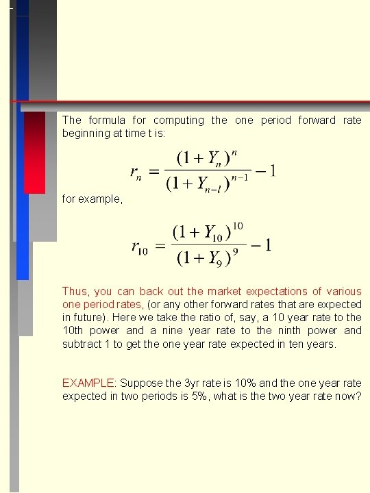
The formula for computing the one period forward rate beginning at time t is: for example, Thus, you can back out the market expectations of various one period rates, (or any other forward rates that are expected in future). Here we take the ratio of, say, a 10 year rate to the 10 th power and a nine year rate to the ninth power and subtract 1 to get the one year rate expected in ten years. EXAMPLE: Suppose the 3 yr rate is 10% and the one year rate expected in two periods is 5%, what is the two year rate now?

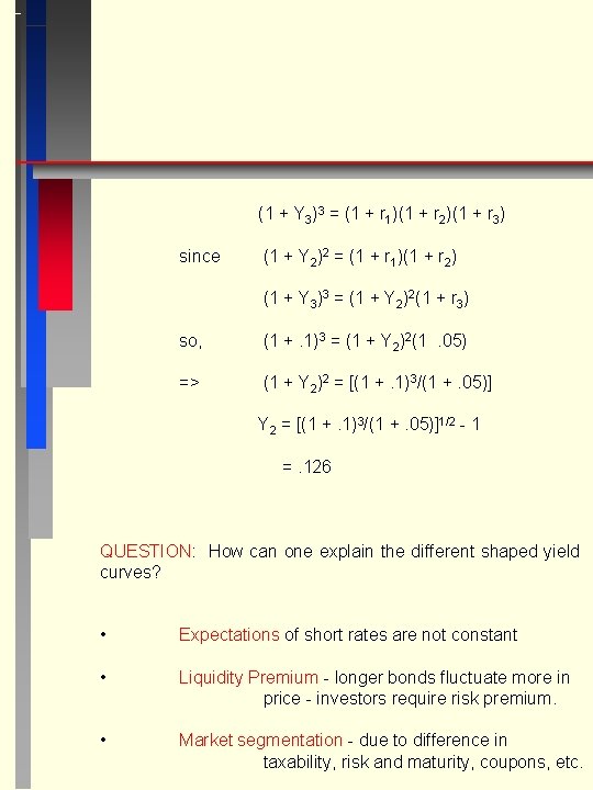
(1 + Y 3)3 = (1 + r 1)(1 + r 2)(1 + r 3) since (1 + Y 2)2 = (1 + r 1)(1 + r 2) (1 + Y 3)3 = (1 + Y 2)2(1 + r 3) so, (1 +. 1)3 = (1 + Y 2)2(1. 05) => (1 + Y 2)2 = [(1 +. 1)3/(1 +. 05)] Y 2 = [(1 +. 1)3/(1 +. 05)]1/2 - 1 =. 126 QUESTION: How can one explain the different shaped yield curves? • Expectations of short rates are not constant • Liquidity Premium - longer bonds fluctuate more in price - investors require risk premium. • Market segmentation - due to difference in taxability, risk and maturity, coupons, etc.

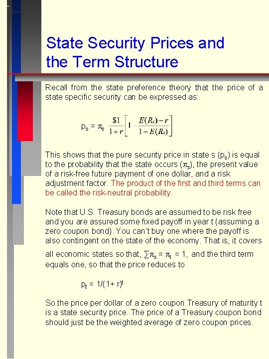
State Security Prices and the Term Structure Recall from the state preference theory that the price of a state specific security can be expressed as: ps = s This shows that the pure security price in state s (ps) is equal to the probability that the state occurs ( s), the present value of a risk-free future payment of one dollar, and a risk adjustment factor. The product of the first and third terms can be called the risk-neutral probability. Note that U. S. Treasury bonds are assumed to be risk free and you are assured some fixed payoff in year t (assuming a zero coupon bond). You can’t buy one where the payoff is also contingent on the state of the economy. That is, it covers all economic states so that, ∑ s = t = 1, and the third term equals one, so that the price reduces to pt = 1/(1+ r)t So the price per dollar of a zero coupon Treasury of maturity t is a state security price. The price of a Treasury coupon bond should just be the weighted average of zero coupon prices.

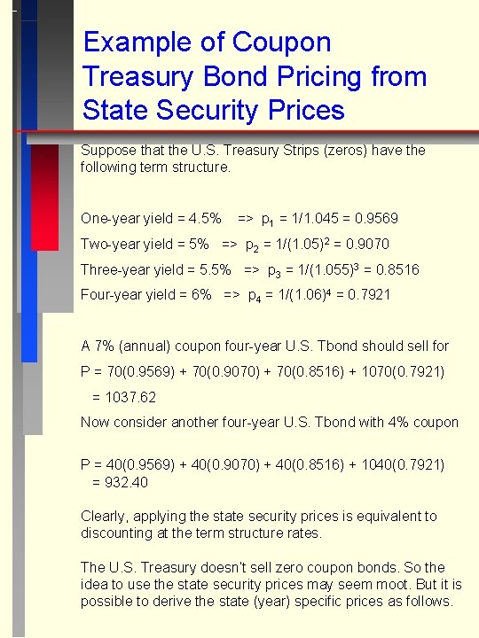
Example of Coupon Treasury Bond Pricing from State Security Prices Suppose that the U. S. Treasury Strips (zeros) have the following term structure. One-year yield = 4. 5% => p 1 = 1/1. 045 = 0. 9569 Two-year yield = 5% => p 2 = 1/(1. 05)2 = 0. 9070 Three-year yield = 5. 5% => p 3 = 1/(1. 055)3 = 0. 8516 Four-year yield = 6% => p 4 = 1/(1. 06)4 = 0. 7921 A 7% (annual) coupon four-year U. S. Tbond should sell for P = 70(0. 9569) + 70(0. 9070) + 70(0. 8516) + 1070(0. 7921) = 1037. 62 Now consider another four-year U. S. Tbond with 4% coupon P = 40(0. 9569) + 40(0. 9070) + 40(0. 8516) + 1040(0. 7921) = 932. 40 Clearly, applying the state security prices is equivalent to discounting at the term structure rates. The U. S. Treasury doesn’t sell zero coupon bonds. So the idea to use the state security prices may seem moot. But it is possible to derive the state (year) specific prices as follows.

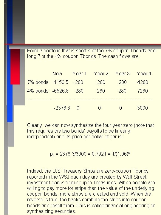
Form a portfolio that is short 4 of the 7% coupon Tbonds and long 7 of the 4% coupon Tbonds. The cash flows are: Now Year 1 Year 2 Year 3 Year 4 4150. 5 -280 -4280 4% bonds -6526. 8 280 280 7% bonds ----------------------------------------2376. 3 0 0 0 3000 Clearly, we can now synthesize the four-year zero (note that this requires the two bonds’ payoffs to be linearly independent) and its price per dollar of par is: p 4 = 2376. 3/3000 = 0. 7921 = 1/(1. 06)4 Indeed, the U. S. Treasury Strips are zero-coupon Tbonds reported in the WSJ each day are created by Wall Street investment banks from coupon Treasuries. When people are willing to pay more for strips than the value of the underlying coupon bonds, more strips are created and sold. When the reverse is true, the banks combine the strips into coupon bonds and resell them. This is called financial engineering or synthesizing securities.

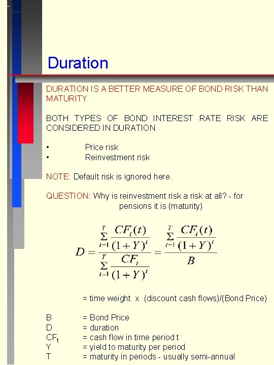
Duration DURATION IS A BETTER MEASURE OF BOND RISK THAN MATURITY BOTH TYPES OF BOND INTEREST RATE RISK ARE CONSIDERED IN DURATION • • Price risk Reinvestment risk NOTE: Default risk is ignored here. QUESTION: Why is reinvestment risk at all? - for pensions it is (maturity) = time weight x (discount cash flows)/(Bond Price) B D CFt Y T = Bond Price = duration = cash flow in time period t = yield to maturity period = maturity in periods - usually semi-annual

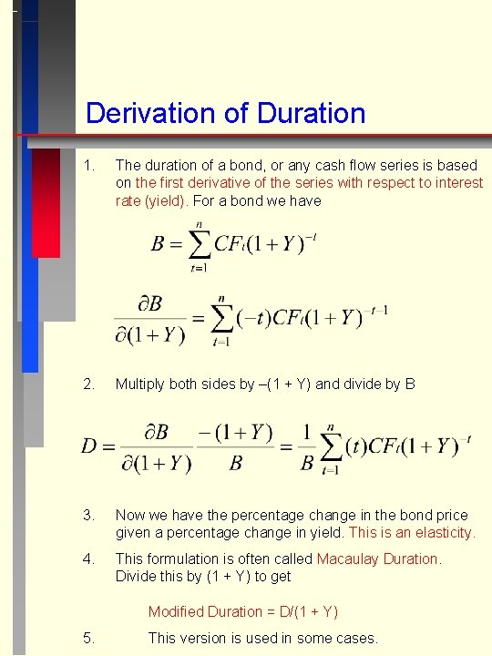
Derivation of Duration 1. The duration of a bond, or any cash flow series is based on the first derivative of the series with respect to interest rate (yield). For a bond we have 2. Multiply both sides by –(1 + Y) and divide by B 3. Now we have the percentage change in the bond price given a percentage change in yield. This is an elasticity. 4. This formulation is often called Macaulay Duration. Divide this by (1 + Y) to get Modified Duration = D/(1 + Y) 5. This version is used in some cases.

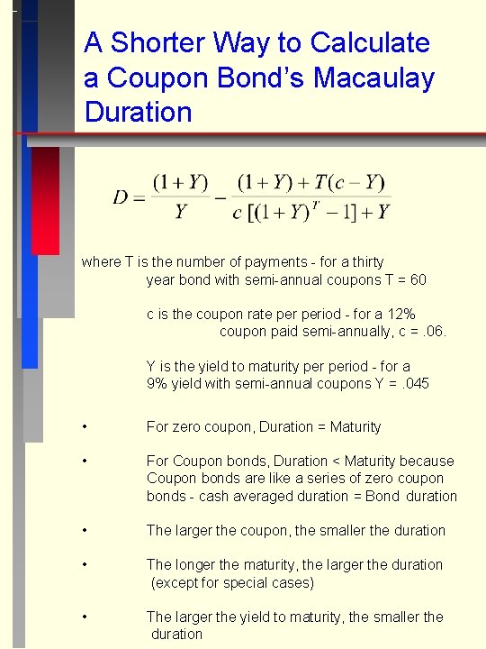
A Shorter Way to Calculate a Coupon Bond’s Macaulay Duration where T is the number of payments - for a thirty year bond with semi-annual coupons T = 60 c is the coupon rate period - for a 12% coupon paid semi-annually, c =. 06. Y is the yield to maturity period - for a 9% yield with semi-annual coupons Y =. 045 • For zero coupon, Duration = Maturity • For Coupon bonds, Duration < Maturity because Coupon bonds are like a series of zero coupon bonds - cash averaged duration = Bond duration • The larger the coupon, the smaller the duration • The longer the maturity, the larger the duration (except for special cases) • The larger the yield to maturity, the smaller the duration

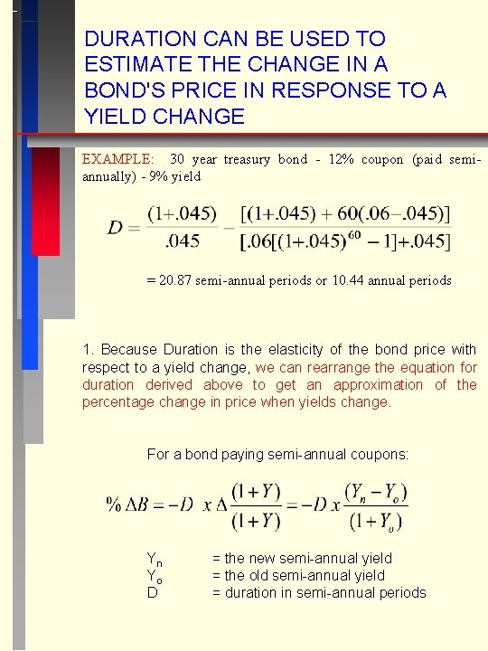
DURATION CAN BE USED TO ESTIMATE THE CHANGE IN A BOND'S PRICE IN RESPONSE TO A YIELD CHANGE EXAMPLE: 30 year treasury bond - 12% coupon (paid semiannually) - 9% yield = 20. 87 semi-annual periods or 10. 44 annual periods 1. Because Duration is the elasticity of the bond price with respect to a yield change, we can rearrange the equation for duration derived above to get an approximation of the percentage change in price when yields change. For a bond paying semi-annual coupons: Yn Yo D = the new semi-annual yield = the old semi-annual yield = duration in semi-annual periods

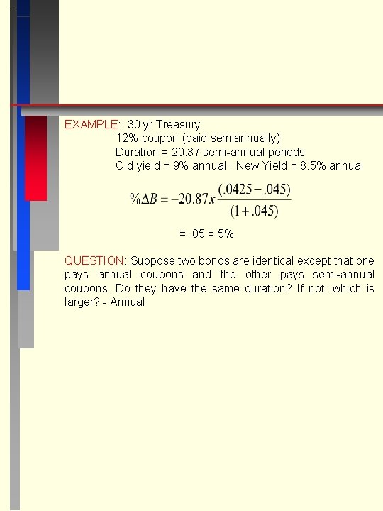
EXAMPLE: 30 yr Treasury 12% coupon (paid semiannually) Duration = 20. 87 semi-annual periods Old yield = 9% annual - New Yield = 8. 5% annual =. 05 = 5% QUESTION: Suppose two bonds are identical except that one pays annual coupons and the other pays semi-annual coupons. Do they have the same duration? If not, which is larger? - Annual

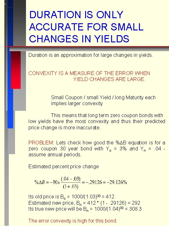
DURATION IS ONLY ACCURATE FOR SMALL CHANGES IN YIELDS Duration is an approximation for large changes in yields. CONVEXITY IS A MEASURE OF THE ERROR WHEN YIELD CHANGES ARE LARGE. Small Coupon / small Yield / long Maturity each implies larger convexity This means that long term zero coupon bonds with low yields have the most convexity and thus their predicted price change is more inaccurate. PROBLEM: Lets check how good the % B equation is for a zero coupon 30 year bond with Yo = 3% and Yn =. 04 assume annual periods. Estimated percent price change Its old price is Bo = 1000/(1. 03)30 = 412. Estimated new price, Bn = 412 * (1 -. 29126) = 292 Its true new price will be Bn = 1000/(1. 04)30 = 308. 3 The error convexity is high for this bond.

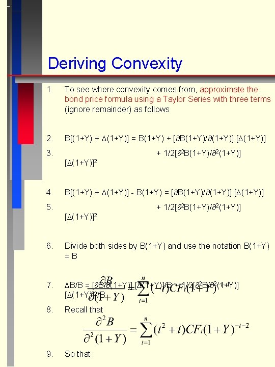
Deriving Convexity 1. To see where convexity comes from, approximate the bond price formula using a Taylor Series with three terms (ignore remainder) as follows 2. B[(1+Y) + (1+Y)] = B(1+Y) + [ B(1+Y)/ (1+Y)] [ (1+Y)] 3. + 1/2[ 2 B(1+Y)/ 2(1+Y)] [ (1+Y)]2 4. B[(1+Y) + (1+Y)] - B(1+Y) = [ B(1+Y)/ (1+Y)] [ (1+Y)] 5. + 1/2[ 2 B(1+Y)/ 2(1+Y)] [ (1+Y)]2 6. Divide both sides by B(1+Y) and use the notation B(1+Y) =B 7. B/B = [ B/ (1+Y)] [ (1+Y)]/B + 1/2[ 2 B/ 2(1+Y)] [ (1+Y)]2/B 8. Recall that 9. So that

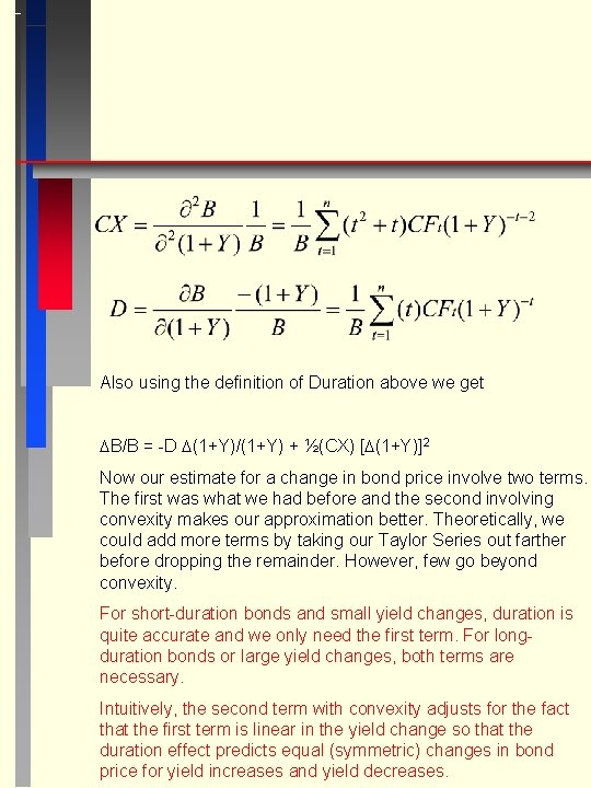
Also using the definition of Duration above we get B/B = -D (1+Y)/(1+Y) + ½(CX) [ (1+Y)]2 Now our estimate for a change in bond price involve two terms. The first was what we had before and the second involving convexity makes our approximation better. Theoretically, we could add more terms by taking our Taylor Series out farther before dropping the remainder. However, few go beyond convexity. For short-duration bonds and small yield changes, duration is quite accurate and we only need the first term. For longduration bonds or large yield changes, both terms are necessary. Intuitively, the second term with convexity adjusts for the fact that the first term is linear in the yield change so that the duration effect predicts equal (symmetric) changes in bond price for yield increases and yield decreases.

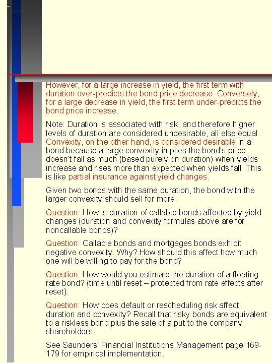
However, for a large increase in yield, the first term with duration over-predicts the bond price decrease. Conversely, for a large decrease in yield, the first term under-predicts the bond price increase. Note: Duration is associated with risk, and therefore higher levels of duration are considered undesirable, all else equal. Convexity, on the other hand, is considered desirable in a bond because a large convexity implies the bond’s price doesn’t fall as much (based purely on duration) when yields increase and rises more than expected when yields fall. This is like partial insurance against yield changes. Given two bonds with the same duration, the bond with the larger convexity should sell for more. Question: How is duration of callable bonds affected by yield changes (duration and convexity formulas above are for noncallable bonds)? Question: Callable bonds and mortgages bonds exhibit negative convexity. Why? How should this affect how much one will be willing to pay for the bond? Question: How would you estimate the duration of a floating rate bond? (time until reset – protected from rate effects after reset). Question: How does default or rescheduling risk affect duration and convexity? Recall that risky bonds are equivalent to a riskless bond plus the sale of a put to the company shareholders. See Saunders’ Financial Institutions Management page 169179 for empirical implementation.

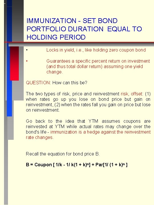
IMMUNIZATION - SET BOND PORTFOLIO DURATION EQUAL TO HOLDING PERIOD • Locks in yield, i. e. , like holding zero coupon bond • Guarantees a specific percent return on investment (and thus total dollar return) assuming one yield change. QUESTION: How can this be? The two types of risk, price and reinvestment risk, offset: (1) when rates go up you lose on bond price but gain on reinvestment, (2) when the rates fall you gain on price but lose on reinvestment. Go back to the idea that YTM assumes coupons are reinvested at YTM while actual rates may change over the bond's life - immunization is a hedge against the reinvestment rate changes. Recall the equation for bond price B. B = Coupon [ 1/k - 1/ k(1 + k)n] + Par[1/ (1 + k)n ]

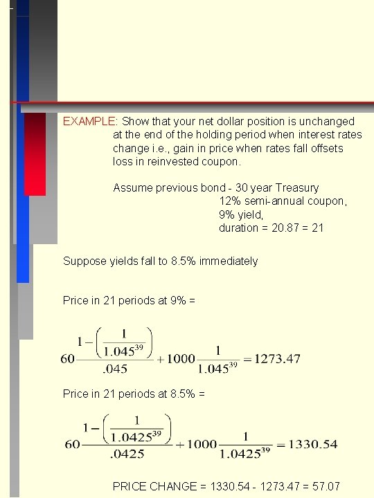
EXAMPLE: Show that your net dollar position is unchanged at the end of the holding period when interest rates change i. e. , gain in price when rates fall offsets loss in reinvested coupon. Assume previous bond - 30 year Treasury 12% semi-annual coupon, 9% yield, duration = 20. 87 = 21 Suppose yields fall to 8. 5% immediately Price in 21 periods at 9% = Price in 21 periods at 8. 5% = PRICE CHANGE = 1330. 54 - 1273. 47 = 57. 07

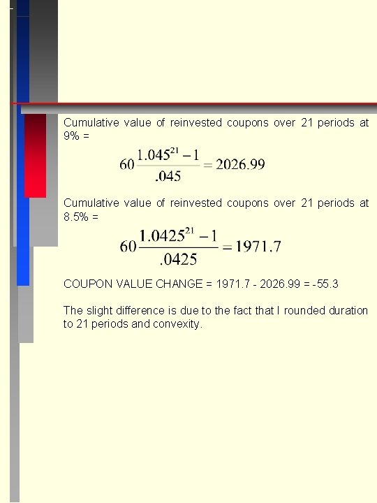
Cumulative value of reinvested coupons over 21 periods at 9% = Cumulative value of reinvested coupons over 21 periods at 8. 5% = COUPON VALUE CHANGE = 1971. 7 - 2026. 99 = -55. 3 The slight difference is due to the fact that I rounded duration to 21 periods and convexity.

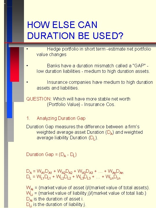
HOW ELSE CAN DURATION BE USED? • Hedge portfolio in short term -estimate net portfolio value changes • Banks have a duration mismatch called a "GAP" low duration liabilities - medium to high duration assets. • Insurance companies have medium to high duration assets and liabilities. QUESTION: Which will have more stable net worth (Portfolio Value) - Insurance Cos. 1. Analyzing Duration Gap measures the difference between a firm’s weighted average asset Duration (DA) and weighted average liability Duration (DL). Duration Gap = (DA - DL) DA = WA 1 DA 1 + WA 2 DA 2 + WA 3 DA 3 + … + WAn. DAn DL = WL 1 DL 1 + WL 2 DL 2 + WL 3 DL 3 + … + WLn. DLn WAi = (market value of asset i)/(market value of total assets). WLi = (market value of liability j)/(market value of total liab. ) DAi is the duration of asset i. DLi is the duration of liability j.

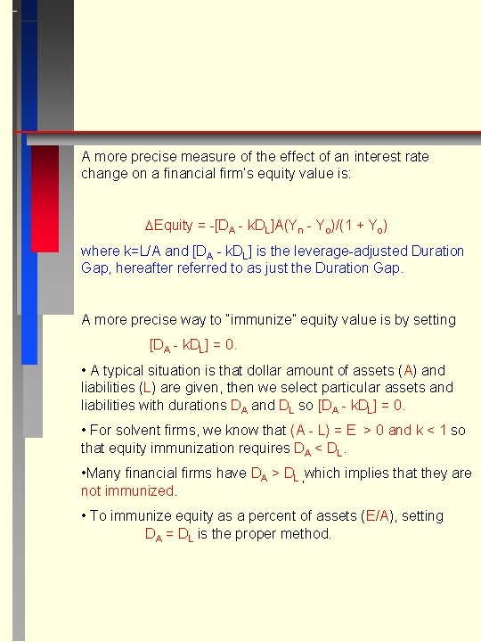
A more precise measure of the effect of an interest rate change on a financial firm’s equity value is: Equity = -[DA - k. DL]A(Yn - Yo)/(1 + Yo) where k=L/A and [DA - k. DL] is the leverage-adjusted Duration Gap, hereafter referred to as just the Duration Gap. A more precise way to “immunize” equity value is by setting [DA - k. DL] = 0. • A typical situation is that dollar amount of assets (A) and liabilities (L) are given, then we select particular assets and liabilities with durations DA and DL so [DA - k. DL] = 0. • For solvent firms, we know that (A - L) = E > 0 and k < 1 so that equity immunization requires DA < DL. • Many financial firms have DA > DL , which implies that they are not immunized. • To immunize equity as a percent of assets (E/A), setting DA = DL is the proper method.

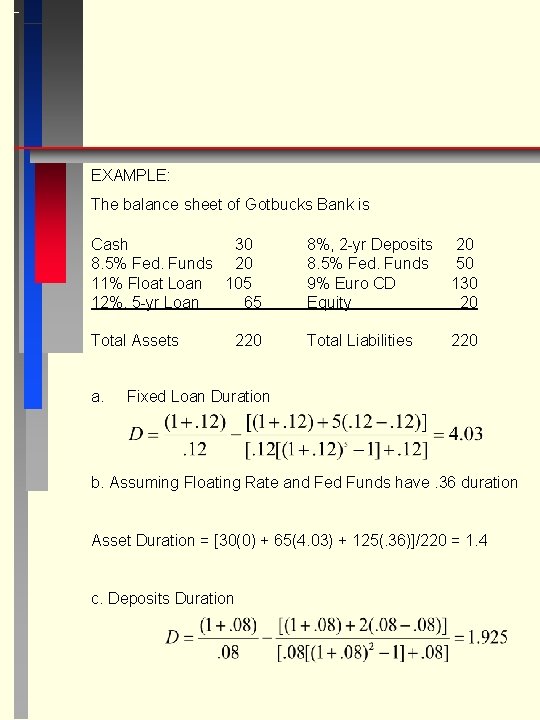
EXAMPLE: The balance sheet of Gotbucks Bank is Cash 30 8. 5% Fed. Funds 20 11% Float Loan 105 12%, 5 -yr Loan 65 8%, 2 -yr Deposits 8. 5% Fed. Funds 9% Euro CD Equity 20 50 130 20 Total Assets Total Liabilities 220 a. 220 Fixed Loan Duration b. Assuming Floating Rate and Fed Funds have. 36 duration Asset Duration = [30(0) + 65(4. 03) + 125(. 36)]/220 = 1. 4 c. Deposits Duration

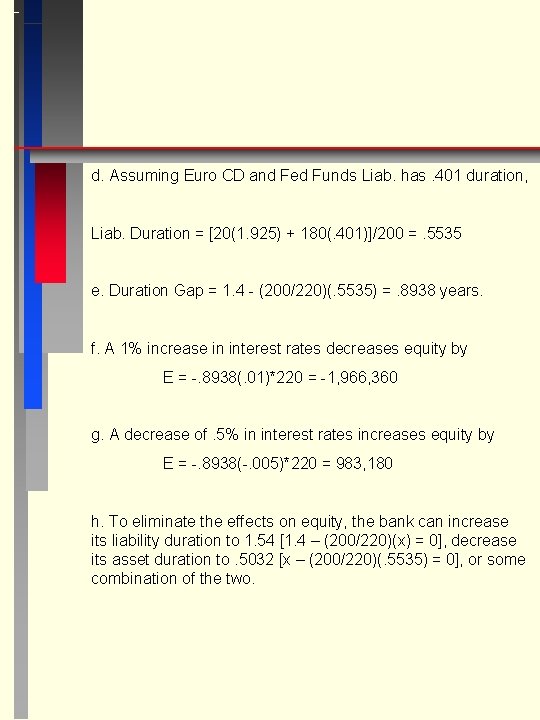
d. Assuming Euro CD and Fed Funds Liab. has. 401 duration, Liab. Duration = [20(1. 925) + 180(. 401)]/200 =. 5535 e. Duration Gap = 1. 4 - (200/220)(. 5535) =. 8938 years. f. A 1% increase in interest rates decreases equity by E = -. 8938(. 01)*220 = -1, 966, 360 g. A decrease of. 5% in interest rates increases equity by E = -. 8938(-. 005)*220 = 983, 180 h. To eliminate the effects on equity, the bank can increase its liability duration to 1. 54 [1. 4 – (200/220)(x) = 0], decrease its asset duration to. 5032 [x – (200/220)(. 5535) = 0], or some combination of the two.

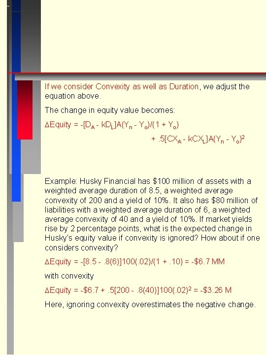
If we consider Convexity as well as Duration, we adjust the equation above. The change in equity value becomes: Equity = -[DA - k. DL]A(Yn - Yo)/(1 + Yo) +. 5[CXA - k. CXL]A(Yn - Yo)2 Example: Husky Financial has $100 million of assets with a weighted average duration of 8. 5, a weighted average convexity of 200 and a yield of 10%. It also has $80 million of liabilities with a weighted average duration of 6, a weighted average convexity of 40 and a yield of 10%. If market yields rise by 2 percentage points, what is the expected change in Husky’s equity value if convexity is ignored? How about if one considers convexity? Equity = -[8. 5 -. 8(6)]100(. 02)/(1 +. 10) = -$6. 7 MM with convexity Equity = -$6. 7 +. 5[200 -. 8(40)]100(. 02)2 = -$3. 26 M Here, ignoring convexity overestimates the negative change.