XML XML Structure of XML Data XML Document


 Derived")
 The ability to specify new tags, and to create nested")

 Earlier generation formats were based on plain text with line")


 Mixture of text with sub-elements is legal in")


 The type of an XML document can be specified using")

+)> <!ELEMENT department ( dept name,")


 <xs: complex. Type name=“University. Type”>")


 parts of documents using path expressions A")
 The initial “/” denotes root of the document (above the toplevel")
 at the end of")
![MORE XPATH FEATURES Operator “|” used to implement union E. g. /university-3/course[@dept name=“Comp. Sci”]](https://slidetodoc.com/presentation_image_h2/49c64fcd943286efaa550f74877facb2/image-34.jpg "MORE XPATH FEATURES Operator “|” used to implement union E. g. /university-3/course[@dept name=“Comp. Sci”]")


 Older browsers without the support for the Java. Script function JSON. parse()")
 method compiles and executes the given string The string")


 HBase is based on Google’s Bigtable model")
 § § § HBase schema consists of")

")


 Assigns regions, detects")


![CREATE TABLE create '<tablename>' , {NAME => '<colfam>' [, <options>]} [, {…}] create 't](https://slidetodoc.com/presentation_image_h2/49c64fcd943286efaa550f74877facb2/image-93.jpg "CREATE TABLE create '<tablename>' , {NAME => '<colfam>' [, <options>]} [, {…}] create 't")
![ACCESSING DATA IN TABLES Get get '<tablename>', '<rowkey>' [, options] – get 't 1',](https://slidetodoc.com/presentation_image_h2/49c64fcd943286efaa550f74877facb2/image-94.jpg "ACCESSING DATA IN TABLES Get get '<tablename>', '<rowkey>' [, options] – get 't 1',")
![SCAN AND COUNT Scan: scan '<tablename>' [, {<options>}] – May include options for COLUMNS,](https://slidetodoc.com/presentation_image_h2/49c64fcd943286efaa550f74877facb2/image-95.jpg "SCAN AND COUNT Scan: scan '<tablename>' [, {<options>}] – May include options for COLUMNS,")


 Complex type: List / Map")


")


 Began life in 1991 as a dynamic linear")
 In 1996, Seltzer and Bostic started Sleepycat Software.")
 Berkeley DB 4. 0, Released in 1999 Single-Master,")


 feature set 1. Most similar to the")


")


")
')")


', ylab='Weight Gain', names =")
![BOXPLOT GROUPINGS Do it by shift wg. 7 a <- D[D$Shift=="7 am", ] wg.](https://slidetodoc.com/presentation_image_h2/49c64fcd943286efaa550f74877facb2/image-154.jpg "BOXPLOT GROUPINGS Do it by shift wg. 7 a <- D[D$Shift==\"7 am\", ] wg.")


', ylab='Weight Gain (lbs)')")
', ylab='Weight Gain (lbs)', pch=2)")


")
)")


- Slides: 166
XML
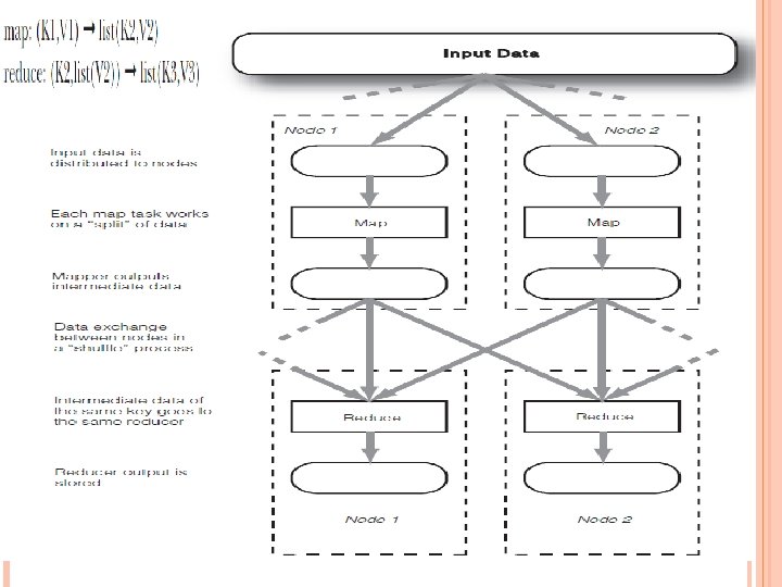
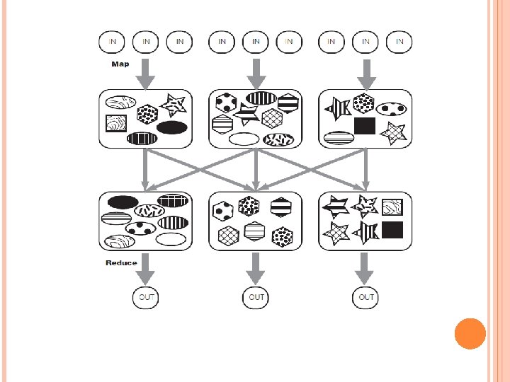
XML Structure of XML Data XML Document Schema Querying and Transformation
INTRODUCTION XML: Extensible Markup Language Defined by the WWW Consortium (W 3 C) Derived from SGML (Standard Generalized Markup Language), but simpler to use than SGML Documents have tags giving extra information about sections of the document E. g. <title> XML </title> <slide> Introduction …</slide> Extensible, unlike HTML Users can add new tags, and separately specify how the tag should be handled for display
XML INTRODUCTION (CONT. ) The ability to specify new tags, and to create nested tag structures make XML a great way to exchange data, not just documents. Much of the use of XML has been in data exchange applications, not as a replacement for HTML Tags make data (relatively) self-documenting E. g. <university> <department> <dept_name> Comp. Sci. </dept_name> <building> Taylor </building> <budget> 100000 </budget> </department> <course_id> CS-101 </course_id> <title> Intro. to Computer Science </title> <dept_name> Comp. Sci </dept_name> <credits> 4 </credits> </course> </university>
XML: MOTIVATION Data interchange is critical in today’s networked world Examples: Banking: funds transfer Order processing (especially inter-company orders) Scientific data Chemistry: Chem. ML, … Genetics: BSML (Bio-Sequence Markup Language), … Paper flow of information between organizations is being replaced by electronic flow of information Each application area has its own set of standards for representing information XML has become the basis for all new generation data interchange formats
XML MOTIVATION (CONT. ) Earlier generation formats were based on plain text with line headers indicating the meaning of fields Similar in concept to email headers Does not allow for nested structures, no standard “type” language Tied too closely to low level document structure (lines, spaces, etc) Each XML based standard defines what are valid elements, using XML type specification languages to specify the syntax DTD (Document Type Descriptors) XML Schema XML allows new tags to be defined as required Plus textual descriptions of the semantics However, this may be constrained by DTDs A wide variety of tools is available for parsing, browsing and querying XML documents/data
COMPARISON WITH RELATIONAL DATA Inefficient: tags, which in effect represent schema information, are repeated Better than relational tuples as a data-exchange format Unlike relational tuples, XML data is self-documenting due to presence of tags Non-rigid format: tags can be added Allows nested structures Wide acceptance, not only in database systems, but also in browsers, tools, and applications
STRUCTURE OF XML DATA Tag: label for a section of data Element: section of data beginning with <tagname> and ending with matching </tagname> Elements must be properly nested Proper nesting <course> … <title> …. </title> </course> Improper nesting <course> … <title> …. </course> </title> Formally: every start tag must have a unique matching end tag, that is in the context of the same parent element. Every document must have a single top-level element
EXAMPLE OF NESTED ELEMENTS <purchase_order> <identifier> P-101 </identifier> <purchaser> …. </purchaser> <itemlist> <item> <identifier> RS 1 </identifier> <description> Atom powered rocket sled </description> <quantity> 2 </quantity> <price> 199. 95 </price> </item> <identifier> SG 2 </identifier> <description> Superb glue </description> <quantity> 1 </quantity> <unit-of-measure> liter </unit-of-measure> <price> 29. 95 </price> </itemlist> </purchase_order>
MOTIVATION FOR NESTING Nesting of data is useful in data transfer Example: elements representing item nested within an itemlist Nesting is not supported, or discouraged, in relational databases With multiple orders, customer name and address are stored redundantly normalization replaces nested structures in each order by foreign key into table storing customer name and address information Nesting is supported in object-relational databases But nesting is appropriate when transferring data External application does not have direct access to data referenced by a foreign key
STRUCTURE OF XML DATA (CONT. ) Mixture of text with sub-elements is legal in XML. Example: <course> This course is being offered for the first time in 2009. <course id> BIO-399 </course id> <title> Computational Biology </title> <dept name> Biology </dept name> <credits> 3 </credits> </course> Useful for document markup, but discouraged for data representation
ATTRIBUTES Elements can have attributes <course_id= “CS-101”> <title> Intro. to Computer Science</title> <dept name> Comp. Sci. </dept name> <credits> 4 </credits> </course> Attributes are specified by name=value pairs inside the starting tag of an element An element may have several attributes, but each attribute name can only occur once <course_id = “CS-101” credits=“ 4”>
ATTRIBUTES VS. SUBELEMENTS Distinction between subelement and attribute In the context of documents, attributes are part of markup, while subelement contents are part of the basic document contents In the context of data representation, the difference is unclear and may be confusing Same information can be represented in two ways <course_id= “CS-101”> … </course> <course> <course_id>CS-101</course_id> … </course> Suggestion: use attributes for identifiers of elements, and use subelements for contents
NAMESPACES XML data has to be exchanged between organizations Same tag name may have different meaning in different organizations, causing confusion on exchanged documents Specifying a unique string as an element name avoids confusion Better solution: use unique-name: element-name Avoid using long unique names all over document by using XML Namespaces <university xmlns: yale=“http: //www. yale. edu”> … <yale: course> <yale: course_id> CS-101 </yale: course_id> <yale: title> Intro. to Computer Science</yale: title> <yale: dept_name> Comp. Sci. </yale: dept_name> <yale: credits> 4 </yale: credits> </yale: course> … </university>
MORE ON XML SYNTAX Elements without subelements or text content can be abbreviated by ending the start tag with a /> and deleting the end tag <course_id=“CS-101” Title=“Intro. To Computer Science” dept_name = “Comp. Sci. ” credits=“ 4” /> To store string data that may contain tags, without the tags being interpreted as subelements, use CDATA as below <![CDATA[<course> … </course>]]> Here, <course> and </course> are treated as just strings CDATA stands for “character data”
XML DOCUMENT SCHEMA Database schemas constrain what information can be stored, and the data types of stored values XML documents are not required to have an associated schema However, schemas are very important for XML data exchange Otherwise, a site cannot automatically interpret data received from another site Two mechanisms for specifying XML schema Document Type Widely used Definition (DTD) XML Schema Newer, increasing use
DOCUMENT TYPE DEFINITION (DTD) The type of an XML document can be specified using a DTD constraints structure of XML data What elements can occur What attributes can/must an element have What subelements can/must occur inside each element, and how many times. DTD does not constrain data types All values represented as strings in XML DTD syntax <!ELEMENT element (subelements-specification) > <!ATTLIST element (attributes) >
ELEMENT SPECIFICATION IN DTD Subelements can be specified as names of elements, or #PCDATA (parsed character data), i. e. , character strings EMPTY (no subelements) or ANY (anything can be a subelement) Example <! ELEMENT department (dept_name building, budget)> <! ELEMENT dept_name (#PCDATA)> <! ELEMENT budget (#PCDATA)> Subelement specification may have regular expressions <!ELEMENT university ( ( department | course | instructor | teaches )+)> Notation: “|” - alternatives “+” - 1 or more occurrences “*” - 0 or more occurrences
UNIVERSITY DTD <!DOCTYPE university [ <!ELEMENT university ( (department|course|instructor|teaches)+)> <!ELEMENT department ( dept name, building, budget)> <!ELEMENT course ( course id, title, dept name, credits)> <!ELEMENT instructor (IID, name, dept name, salary)> <!ELEMENT teaches (IID, course id)> <!ELEMENT dept name( #PCDATA )> <!ELEMENT building( #PCDATA )> <!ELEMENT budget( #PCDATA )> <!ELEMENT course id ( #PCDATA )> <!ELEMENT title ( #PCDATA )> <!ELEMENT credits( #PCDATA )> <!ELEMENT IID( #PCDATA )> <!ELEMENT name( #PCDATA )> <!ELEMENT salary( #PCDATA )> ]>
ATTRIBUTE SPECIFICATION IN DTD Attribute specification : for each attribute Name Type of attribute CDATA ID (identifier) or IDREF (ID reference) or IDREFS (multiple IDREFs) more on this later Whether mandatory (#REQUIRED) has a default value (value), or neither (#IMPLIED) Examples <!ATTLIST course_id CDATA #REQUIRED>, or <!ATTLIST course_id ID #REQUIRED dept_name IDREF #REQUIRED instructors IDREFS #IMPLIED >
IDS AND IDREFS An element can have at most one attribute of type ID The ID attribute value of each element in an XML document must be distinct Thus the ID attribute value is an object identifier An attribute of type IDREF must contain the ID value of an element in the same document An attribute of type IDREFS contains a set of (0 or more) ID values. Each ID value must contain the ID value of an element in the same document
UNIVERSITY DTD WITH ATTRIBUTES University DTD with ID and IDREF attribute types. <!DOCTYPE university-3 [ <!ELEMENT university ( (department|course|instructor)+)> <!ELEMENT department ( building, budget )> <!ATTLIST department dept_name ID #REQUIRED > <!ELEMENT course (title, credits )> <!ATTLIST course_id ID #REQUIRED dept_name IDREF #REQUIRED instructors IDREFS #IMPLIED > <!ELEMENT instructor ( name, salary )> <!ATTLIST instructor IID ID #REQUIRED dept_name IDREF #REQUIRED > · · · declarations for title, credits, building, budget, name and salary · · · ]>
XML DATA WITH ID AND IDREF ATTRIBUTES <university-3> <department dept name=“Comp. Sci. ”> <building> Taylor </building> <budget> 100000 </budget> </department> <department dept name=“Biology”> <building> Watson </building> <budget> 90000 </budget> </department> <course id=“CS-101” dept name=“Comp. Sci” instructors=“ 10101 83821”> <title> Intro. to Computer Science </title> <credits> 4 </credits> </course> …. <instructor IID=“ 10101” dept name=“Comp. Sci. ”> <name> Srinivasan </name> <salary> 65000 </salary> </instructor> …. </university-3>
LIMITATIONS OF DTDS No typing of text elements and attributes All values are strings, no integers, reals, etc. Difficult to specify unordered sets of subelements Order is usually irrelevant in databases (unlike in the document-layout environment from which XML evolved) (A | B)* allows specification of an unordered set, but Cannot ensure that each of A and B occurs only once IDs and IDREFs are untyped The instructors attribute of an course may contain a reference to another course, which is meaningless instructors attribute should ideally be constrained to refer to instructor elements
XML SCHEMA XML Schema is a more sophisticated schema language which addresses the drawbacks of DTDs. Supports Typing of values E. g. integer, string, etc Also, constraints on min/max values User-defined, comlex types Many more features, including XML Schema is itself specified in XML syntax, unlike DTDs uniqueness and foreign key constraints, inheritance More-standard representation, but verbose XML Scheme is integrated with namespaces BUT: XML Schema is significantly more complicated than DTDs.
XML SCHEMA VERSION OF UNIV. DTD <xs: schema xmlns: xs=“http: //www. w 3. org/2001/XMLSchema”> <xs: element name=“university” type=“university. Type” /> <xs: element name=“department”> <xs: complex. Type> <xs: sequence> <xs: element name=“dept name” type=“xs: string”/> <xs: element name=“building” type=“xs: string”/> <xs: element name=“budget” type=“xs: decimal”/> </xs: sequence> </xs: complex. Type> </xs: element> …. <xs: element name=“instructor”> <xs: complex. Type> <xs: sequence> <xs: element name=“IID” type=“xs: string”/> <xs: element name=“name” type=“xs: string”/> <xs: element name=“dept name” type=“xs: string”/> <xs: element name=“salary” type=“xs: decimal”/> </xs: sequence> </xs: complex. Type> </xs: element> … Contd.
XML SCHEMA VERSION OF UNIV. DTD …. (CONT. ) <xs: complex. Type name=“University. Type”> <xs: sequence> <xs: element ref=“department” min. Occurs=“ 0” max. Occurs=“unbounded”/> <xs: element ref=“course” min. Occurs=“ 0” max. Occurs=“unbounded”/> <xs: element ref=“instructor” min. Occurs=“ 0” max. Occurs=“unbounded”/> <xs: element ref=“teaches” min. Occurs=“ 0” max. Occurs=“unbounded”/> </xs: sequence> </xs: complex. Type> </xs: schema> n Choice of “xs: ” was ours -- any other namespace prefix could be chosen n Element “university” has type “university. Type”, which is defined separately l xs: complex. Type is used later to create the named complex type “University. Type”
MORE FEATURES OF XML SCHEMA Attributes specified by xs: attribute tag: <xs: attribute name = “dept_name”/> adding the attribute use = “required” means value must be specified Key constraint: “department names form a key for department elements under the root university element: <xs: key name = “dept. Key”> <xs: selector xpath = “/university/department”/> <xs: field xpath = “dept_name”/> <xs: key> Foreign key constraint from course to department: <xs: keyref name = “course. Dept. FKey” refer=“dept. Key”> <xs: selector xpath = “/university/course”/> <xs: field xpath = “dept_name”/> <xs: keyref>
QUERYING AND TRANSFORMING XML DATA Translation of information from one XML schema to another Querying on XML data Above two are closely related, and handled by the same tools Standard XML querying/translation languages XPath Simple language consisting of path expressions XSLT Simple language designed for translation from XML to XML and XML to HTML XQuery An XML query language with a rich set of features
TREE MODEL OF XML DATA Query and transformation languages are based on a tree model of XML data An XML document is modeled as a tree, with nodes corresponding to elements and attributes Element nodes have child nodes, which can be attributes or subelements Text in an element is modeled as a text node child of the element Children of a node are ordered according to their order in the XML document Element and attribute nodes (except for the root node) have a single parent, which is an element node The root node has a single child, which is the root element of the document
XPATH XPath is used to address (select) parts of documents using path expressions A path expression is a sequence of steps separated by “/” Think of file names in a directory hierarchy Result of path expression: set of values that along with their containing elements/attributes match the specified path E. g. /university-3/instructor/name evaluated on the university-3 data we saw earlier returns <name>Srinivasan</name> <name>Brandt</name> E. g. /university-3/instructor/name/text( ) returns the same names, but without the enclosing tags
XPATH (CONT. ) The initial “/” denotes root of the document (above the toplevel tag) Path expressions are evaluated left to right Each step operates on the set of instances produced by the previous step Selection predicates may follow any step in a path, in [ ] E. g. /university-3/course[credits >= 4] returns account elements with a balance value greater than 400 /university-3/course[credits] returns account elements containing a credits subelement Attributes are accessed using “@” E. g. /university-3/course[credits >= 4]/@course_id returns the course identifiers of courses with credits >= 4 IDREF attributes are not dereferenced automatically (more on this later)
FUNCTIONS IN XPATH XPath provides several functions The function count() at the end of a path counts the number of elements in the set generated by the path E. g. /university-2/instructor[count(. /teaches/course)> 2] Returns instructors teaching more than 2 courses (on university-2 schema) Also function for testing position (1, 2, . . ) of node w. r. t. siblings Boolean connectives and or and function not() can be used in predicates IDREFs can be referenced using function id() can also be applied to sets of references such as IDREFS and even to strings containing multiple references separated by blanks E. g. /university-3/course/id(@dept_name) returns all department elements referred to from the dept_name attribute of course elements.
MORE XPATH FEATURES Operator “|” used to implement union E. g. /university-3/course[@dept name=“Comp. Sci”] | /university-3/course[@dept name=“Biology”] Gives union of Comp. Sci. and Biology courses However, “|” cannot be nested inside other operators. “//” can be used to skip multiple levels of nodes E. g. /university-3//name finds any name element anywhere under the /university-3 element, regardless of the element in which it is contained. A step in the path can go to parents, siblings, ancestors and descendants of the nodes generated by the previous step, not just to the children “//”, described above, is a short from for specifying “all descendants” “. . ” specifies the parent. doc(name) returns the root of a named document
XQUERY XQuery is a general purpose query language for XML data Currently being standardized by the World Wide Web Consortium (W 3 C) The textbook description is based on a January 2005 draft of the standard. The final version may differ, but major features likely to stay unchanged. XQuery is derived from the Quilt query language, which itself borrows from SQL, XQL and XML-QL XQuery uses a for … let … where … order by …result … syntax for SQL from where SQL where order by SQL order by result SQL select let allows temporary variables, and has no equivalent in SQL
FLWOR SYNTAX IN XQUERY For clause uses XPath expressions, and variable in for clause ranges over values in the set returned by XPath Simple FLWOR expression in XQuery find all courses with credits > 3, with each result enclosed in an <course_id>. . </course_id> tag for $x in /university-3/course let $course. Id : = $x/@course_id where $x/credits > 3 return <course_id> { $course. Id } </course id> Items in the return clause are XML text unless enclosed in {}, in which case they are evaluated Let clause not really needed in this query, and selection can be done In XPath. Query can be written as: for $x in /university-3/course[credits > 3] return <course_id> { $x/@course_id } </course_id> Alternative notation for constructing elements: return element course_id { element $x/@course_id }
JOINS Joins are specified in a manner very similar to SQL for $c in /university/course, $i in /university/instructor, $t in /university/teaches where $c/course_id= $t/course id and $t/IID = $i/IID return <course_instructor> { $c $i } </course_instructor> The same query can be expressed with the selections specified as XPath selections: for $c in /university/course, $i in /university/instructor, $t in /university/teaches[ $c/course_id= $t/course_id and $t/IID = $i/IID] return <course_instructor> { $c $i } </course_instructor>
NESTED QUERIES The following query converts data from the flat structure for university information into the nested structure used in university-1 <university-1> { for $d in /university/department return <department> { $d/* } { for $c in /university/course[dept name = $d/dept name] return $c } </department> } { for $i in /university/instructor return <instructor> { $i/* } { for $c in /university/teaches[IID = $i/IID] return $c/course id } </instructor> } </university-1> $c/* denotes all the children of the node to which $c is bound, without the enclosing top-level tag
GROUPING AND AGGREGATION Nested queries are used for grouping for $d in /university/department return <department-total-salary> <dept_name> { $d/dept name } </dept_name> <total_salary> { fn: sum( for $i in /university/instructor[dept_name = $d/dept_name] return $i/salary )} </total_salary> </department-total-salary>
SORTING IN XQUERY The order by clause can be used at the end of any expression. E. g. to return instructors sorted by name for $i in /university/instructor order by $i/name return <instructor> { $i/* } </instructor> Use order by $i/name descending to sort in descending order Can sort at multiple levels of nesting (sort departments by dept_name, and by courses sorted to course_id within each department) <university-1> { for $d in /university/department order by $d/dept name return <department> { $d/* } { for $c in /university/course[dept name = $d/dept name] order by $c/course id return <course> { $c/* } </course> } </department> } </university-1>
FUNCTIONS AND OTHER XQUERY FEATURES User defined functions with the type system of XMLSchema declare function local: dept_courses($iid as xs: string) as element(course)* { for $i in /university/instructor[IID = $iid], $c in /university/courses[dept_name = $i/dept name] return $c } Types are optional for function parameters and return values The * (as in decimal*) indicates a sequence of values of that type Universal and existential quantification in where clause predicates some $e in path satisfies P every $e in path satisfies P Add and fn: exists($e) to prevent empty $e from satisfying every clause XQuery also supports If-then-else clauses
For example, to find departments where every instructor has a salary greater than $50, 000, we can use the following query: for $d in /university/department where every $i in /university/instructor[dept name=$d/dept name] satisfies $i/salary > 50000 return $d Note, however, that if a department has no instructor, it will trivially satisfy the above condition. An extra clause: and fn: exists(/university/instructor[dept name=$d/dept name])
XSLT A stylesheet stores formatting options for a document, usually separately from document The XML Stylesheet Language (XSL) was originally designed for generating HTML from XML XSLT is a general-purpose transformation language E. g. an HTML style sheet may specify font colors and sizes for headings, etc. Can translate XML to XML, and XML to HTML XSLT transformations are expressed using rules called templates Templates combine selection using XPath with construction of results
END OF XML
JSON JSON: Java. Script Object Notation. syntax for storing and exchanging data. JSON is an easier to use alternative to XML.
JASON JSON is lightweight data interchange format JSON is language independent. JSON is "self-describing" and easy to understand JSON uses Java. Script syntax, but the JSON format is text only, just like XML. Text can be read and used as a data format by any programming language.
JSON Example {"employees": [ {"first. Name": "John", "last. Name": "Doe"}, {"first. Name": "Anna", "last. Name": "Smith"}, {"first. Name": "Peter", "last. Name": "Jones"} ]} XML Example <employees> <employee> <first. Name>John</first. Name> <last. Name>Doe</last. Name> </employee> <first. Name>Anna</first. Name> <last. Name>Smith</last. Name> </employee> <first. Name>Peter</first. Name> <last. Name>Jones</last. Name> </employees>
The JSON format is syntactically identical to the code for creating Java. Script objects. <!DOCTYPE html> <body> <h 2>JSON Object Creation in Java. Script</h 2> <p id="demo"></p> <script> var text = '{"name": "Johnson", "street": "Oslo West 16", "phone": "555 1234567"}' var obj = JSON. parse(text); document. get. Element. By. Id("demo"). inner. HTML =obj. name + " " + obj. street + " " +obj. phone; </script> </body> </html>
LIKE XML Both JSON and XML is plain text Both JSON and XML is "self-describing" (human readable) Both JSON and XML is hierarchical (values within values) Both JSON and XML can be fetched with an Http. Request
UNLIKE XML JSON doesn't use end tag JSON is shorter JSON is quicker to read and write JSON can use arrays The biggest difference is: XML has to be parsed with an XML parser, JSON can be parsed by a standard Java. Script function.
JSON SYNTAX JSON syntax is a subset of the Java. Script object notation syntax: Data is in name/value pairs Data is separated by commas Curly braces hold objects Square brackets hold arrays
JSON DATA - A NAME AND A VALUE JSON data is written as name/value pairs. A name/value pair consists of a field name (in double quotes), followed by a colon, followed by a value: "first. Name": "John“ JSON Values can be: A number (integer or floating point) A string (in double quotes) A Boolean (true or false) An array (in square brackets) An object (in curly braces) null
JSON Objects written inside curly braces. Just like in Java. Script, objects can contain multiple name/values pairs: {"first. Name": "John", "last. Name": "Doe"} JSON Arrays JSON arrays are written inside square brackets. Just like in Java. Script, an array can contain multiple objects: "employees": [ {"first. Name": "John", "last. Name": "Doe"}, {"first. Name": "Anna", "last. Name": "Smith"}, {"first. Name": "Peter", "last. Name": "Jones"} ] In the example above, the object "employees" is an array containing three objects. Each object is a record of a person (with a first name and a last name).
JSON Uses Java. Script Syntax Because JSON uses Java. Script syntax, no extra software is needed to work with JSON within Java. Script. With Java. Script you can create an array of objects and assign data to it like this: Example var employees = [ {"first. Name": "John", "last. Name": "Doe"}, {"first. Name": "Anna", "last. Name": "Smith"}, {"first. Name": "Peter", "last. Name": "Jones"} ]; The first entry in the Java. Script object array can be accessed like this: employees[0]. first. Name + " " + employees[0]. last. Name; The returned content will be: John Doe The data can be modified like this: employees[0]. first. Name = "Gilbert";
A common use of JSON is to read data from a web server, and display the data in a web page. For simplicity, this can be demonstrated by using a string as input. Create a Java. Script string containing JSON syntax: var text = '{ "employees" : [' + '{ "first. Name": "John" , "last. Name": "Doe" }, ' + '{ "first. Name": "Anna" , "last. Name": "Smith" }, ' + '{ "first. Name": "Peter" , "last. Name": "Jones" } ]}'; The Java. Script function JSON. parse(text) can be used to convert a JSON text into a Java. Script object: var obj = JSON. parse(text);
Use the new Java. Script object in your page: Example <p id="demo"></p> <script> document. get. Element. By. Id("demo"). inner. HTML = obj. employees[1]. first. Name + " " + obj. employees[1]. last. Name; </script> Result Create Object from JSON String Anna Smith
USING EVAL() Older browsers without the support for the Java. Script function JSON. parse() can use the eval() function to convert a JSON text into a Java. Script object: var obj = eval ("(" + text + ")");
EVAL The Java. Script eval(string) method compiles and executes the given string The string can be an expression, a statement, or a sequence of statements Expressions can include variables and object properties eval returns the value of the last expression evaluated When applied to JSON, eval returns the described object
BIG DATA
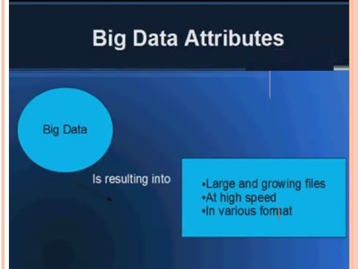
3 VS Velocity Volume Variety.
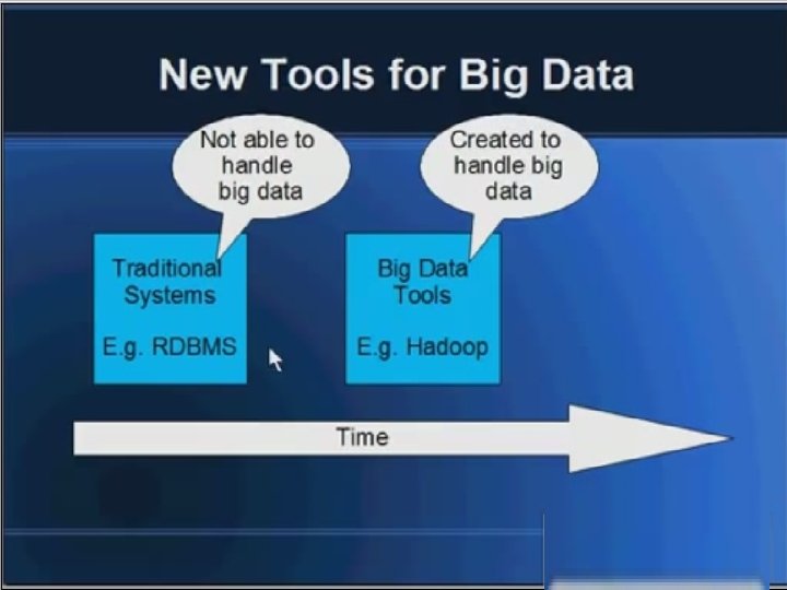
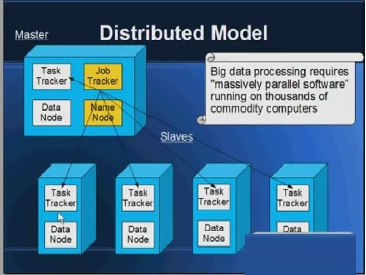
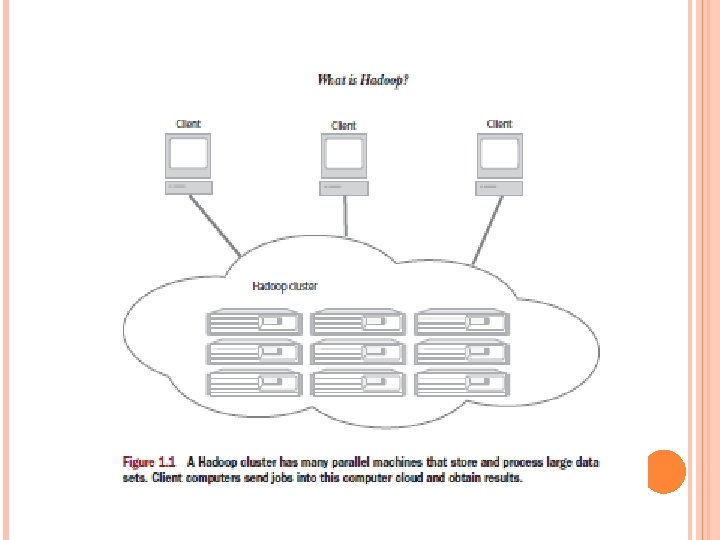
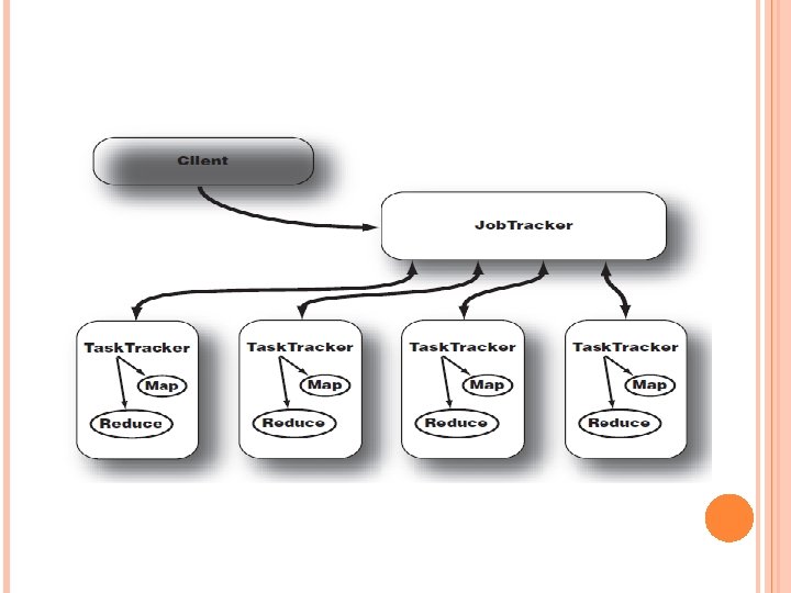
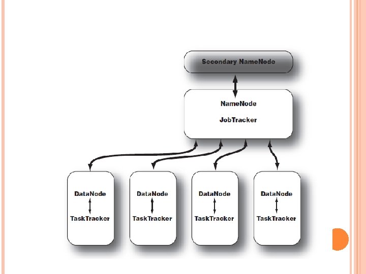
WHAT IS HADOOP Hadoop is an open source framework for writing and running distributed applications that process large amounts of data. Distributed computing is a wide and varied field, but the key distinctions of Hadoop are that it is Accessible Robust Scalable Simple
WHAT IS HBASE? HBase is a distributed column-oriented data store built on top of HDFS HBase is an Apache open source project whose goal is to provide storage for the Hadoop Distributed Computing Data is logically organized into tables, rows and columns § HBase is. . . – Open-Source – Sparse – Multidimensional – Persistent – Distributed – Sorted Map – Runs on top of HDFS – Modeled after Google’s Big. Table
HBASE IS NOT A TRADITIONAL DATABASE
WHEN TO USE HBASE? Use HBase if… – You need random write, random read, or both (but not neither) – You need to do many thousands of operations per second on multiple TB of data – Your access patterns are well-known and simple Don’t use HBase if… – You only append to your dataset, and tend to read the whole thing – Your data easily fits on one beefy node
HBASE DATA MODEL Overview Tables are made of rows and columns Every row has a row key (analogous to a primary key) – Rows are stored sorted by row key for fast lookups All columns in HBase belong to a particular column family A table may have one or more column families – Common to have a small number of column families – Column families should rarely change – A column family can have any number of columns Table cells are versioned, un-interpreted arrays of bytes
HBASE DATA MODEL (CONT …. . ) HBase is based on Google’s Bigtable model Key-Value pairs
HBASE DATA MODEL (CONT …. . ) § § § HBase schema consists of several Tables Each table consists of a set of Column Families Columns are not part of the schema HBase has Dynamic Columns Because column names are encoded inside the cells Different cells can have different columns “Roles” column family has different columns in different cells
HBASE LOGICAL VIEW
HBASE PHYSICAL MODEL Each column family is stored in a separate file (called HTables) Key & Version numbers are replicated with each column family Empty cells are not stored HBase maintains a multi-level index on values: <key, column family, column name, timestamp>
THREE MAJOR COMPONENTS OF HBASE § The HBase. Master - One master § The HRegion. Server - Many region servers § The HBase client
HBASE COMPONENTS Region - A subset of a table’s rows, like horizontal range partitioning - Automatically done Region. Server (many slaves) - Manages data regions - Serves data for reads and writes (using a log) Master - Responsible for coordinating the slaves - Assigns regions, detects failures - Admin functions Zookeeper - A centralized service used to maintain configuration information and service for HBase Catalog Tables - Keep track of the locations of Region. Servers and Regions
HBASE COMPONENTS -- HMASTER Responsible for coordinating the slaves (HRegion. Servers) Assigns regions, detects failures of HRegion. Servers Handles schema changes Master runs several background threads – Load. Balancer Periodically reassigns Regions in the cluster – Catalog. Janitor periodically checks and cleans up the. META. Table Can have multiple Masters – Upon startup all compete to run the cluster – If the active Master loses its lease in Zookeeper then the remaining Masters compete for the Master role
HBASE COMPONENTS -- HREGION SERVERS Serve data for reads and writes of rows contained in Regions Also will split a Region that has become too large Interface Methods exposed by HRegion. Interface – Data Methods, Region Methods – Get, put, delete, next, etc. – split. Region, compact. Region, etc. Runs several background threads – Compact. Split. Thread check for splits, handle minor compactions – Major. Compaction. Checker checks for major compactions – Mem. Store. Flusher periodically flushes in-memory writes in the Mem. Store to Store. Files. – Log. Roller periodically checks the Region. Server's HLog
HBASE COMPONENTS -- REGIONS
HBASE COMPONENTS -- ZOOKEEPER AND CATALOG Zookeeper Service – Stores global information about the cluster – Provides synchronization and detects Master node failure – Holds the location of the -ROOT- table and the Master Catalog -ROOT- Catalog Table – A table that lists the location of the. META. table(s) – The following is an example of: scan ‘-ROOT-’!. META. Catalog Table – A table that lists all the regions and their locations – The following is an example of: scan ‘. META. ’!
HBASE BIG PICTURE
COMPACTION
COMPACTION CONTINUE…. .
RUNNING HBASE SHELL
HBASE – USEFUL COMMANDS help – Lists all the shell commands status – Shows basic status about the cluster list – Lists all user tables in HBase describe '<tablename>' – Returns the structure of the table
CREATE TABLE create '<tablename>' , {NAME => '<colfam>' [, <options>]} [, {…}] create 't 1', {NAME => 'fam 1'} create 't 1', {NAME => 'fam 1', VERSIONS => 1} create 't 1', {NAME => 'fam 1'}, {NAME => 'fam 2'} Shorthand: create 't 1', 'fam 2'
ACCESSING DATA IN TABLES Get get '<tablename>', '<rowkey>' [, options] – get 't 1', 'r 1', {COLUMN => 'fam 1: c 1'} – get 't 1', 'r 1', {COLUMN => 'fam 1: c 1', VERSIONS=> 2} Put put '<tablename>', '<rowkey>', '<colfam>: <col>', '<value>' [, timestamp] – put 't 1', 'r 1', 'fam 1: c 1', 'value', 1274302629663
SCAN AND COUNT Scan: scan '<tablename>' [, {<options>}] – May include options for COLUMNS, START/STOP ROW, TIMESTAMP or COLUMNS – scan 't 1', {COLUMNS => 'fam 1: c 1'} – scan 't 1', {COLUMNS => 'fam 1: '} – scan 't 1', {STARTROW => 'r 1', LIMIT => 10} Count : count '<tablename>' [, interval] – count 't 1', 5000
REMOVING DATA AND TABLES Delete columns in a row – delete '<tablename>', '<row key>', '<col>' – delete 't 1', 'r 1', 'fam 1: c 1' Delete an entire row – deleteall '<tablename>', '<row key>' – deleteall 't 1', 'r 1' Delete all the rows – truncate '<tablename>‘ disable '<tablename>‘ drop '<tablename>‘ major_compact '. META. ’
CHANGING COLUMN FAMILIES Delete columns in a row – delete '<tablename>', '<row key>', '<col>' – delete 't 1', 'r 1', 'fam 1: c 1' Delete an entire row – deleteall '<tablename>', '<row key>' – deleteall 't 1', 'r 1' Delete all the rows – truncate '<tablename>‘ disable '<tablename>‘ drop '<tablename>‘ major_compact '. META. ’
INTRODUCTION TO HIVE
OVERVIEW Intuitive Make the unstructured data looks like tables regardless how it really lay out SQL based query can be directly against these tables Generate specify execution plan for this query What’s Hive A data warehousing system to store structured data on Hadoop file system Provide an easy query these data by execution Hadoop Map. Reduce plans 5/24/2021 Introduction to Hive 99
DATA MODEL Tables Basic type columns (int, float, boolean) Complex type: List / Map ( associate array) Partitions Buckets CREATE TABLE sales( id INT, items ARRAY<STRUCT<id: INT, name: STRING> ) PARITIONED BY (ds STRING) CLUSTERED BY (id) INTO 32 BUCKETS; SELECT id FROM sales TABLESAMPLE (BUCKET 1 OUT 100 OF 32) 5/24/2021 Introduction to Hive
METADATA Database namespace Table definitions schema info, physical location In HDFS Partition data ORM Framework All the metadata can be stored in Derby by default Any database with JDBC can be configed 5/24/2021 Introduction to Hive 101
PERFORMANCE GROUP BY operation Efficient execution plans based on: Data skew: Partial aggregation: 5/24/2021 how evenly distributed data across a number of physical nodes bottleneck VS load balance Group the data with the same group by value as soon as possible In memory hash-table for mapper Earlier than combiner Introduction to Hive 102
PERFORMANCE JOIN operation Traditional Map-Reduce Join Early Map-side Join 7/20/2010 very efficient for joining a small table with a large table Keep smaller table data in memory first Join with a chunk of larger table data each time Space complexity for time complexity Introduction to Hive 103
PERFORMANCE Ser/De Describe how to load the data from the file into a representation that make it looks like a table; Lazy load Create the field object when necessary Reduce the overhead to create unnecessary objects in Hive Java is expensive to create objects Increase performance 7/20/2010 Introduction to Hive 104
HIVE – PERFORMANCE Date SVN Revision Major Changes Query A Query B Query C 2/22/2009 746906 Before Lazy Deserialization 83 sec 98 sec 183 sec 2/23/2009 747293 Lazy Deserialization 40 sec 66 sec 185 sec 3/6/2009 751166 Map-side Aggregation 22 sec 67 sec 182 sec 4/29/2009 770074 Object Reuse 21 sec 49 sec 130 sec 6/3/2009 781633 Map-side Join * 21 sec 48 sec 132 sec 8/5/2009 801497 Lazy Binary Format * 21 sec 48 sec 132 sec Query. A: SELECT count(1) FROM t; Query. B: SELECT concat(concat(a, b), c), d) FROM t; Query. C: SELECT * FROM t; map-side time only (incl. Gzip. Codec for comp/decompression) * These two features need to be tested with other queries. http: //www. slideshare. net/cloudera/hw 09 -hadoop-development-atfacebook-hive-and-hdfs
PROS Pros A easy way to process large scale data Support SQL-based queries Provide more user defined interfaces to extend Programmability Efficient execution plans for performance Interoperability with other database tools 5/24/2021 Introduction to Hive 106
CONS Cons No easy way to append data Files in HDFS are immutable Future work Views / Variables More operator In/Exists semantic More 5/24/2021 future work in the mail list Introduction to Hive 107
APPLICATION Log processing Daily Report User Activity Measurement Data/Text mining Machine learning (Training Data) Business intelligence Advertising Delivery Spam Detection 7/20/2010 Introduction to Hive 108
RELATED WORK Parallel databases: Gamma, Bubba, Volcano Google: Sawzall Yahoo: Pig IBM: JAQL Microsoft: Drad. LINQ , SCOPE 7/20/2010 Introduction to Hive 109
INTRODUCTION TO CLOUDERA
Software organization started in 2009 Open source Hadoop distribution Focuses on distribution of various technologies
PRODUCTS AND SERVICES Annual subscription license Cloudera Express- CDH+ Cloudera manager No roll backs and backup/disaster recovery
Downloaded for free but no technical support
Contains core elements of hadoop Reliable, scalable Distributed data processing of large data sets Security Availability Integration with hardware and software
AN INTRODUCTION TO BERKELEY DB
OVERVIEW OF BERKELEY DB Means the Berkeley Database An open-source, embedded transactional data management system A key/value store Embedded ? As a library that is linked with an application Hides data management from end-user Scales from Bytes to Petabytes Runs on everything from cell phone to large servers.
BERKELEY DB : EXAMPLES OF APPLICATIONS Google Accounts Store all user and service account information and preferences. Amazon’s user-customization Berkeley DB has high reliability and high performance.
BERKELEY DB: A BRIEF HISTORY (1) Began life in 1991 as a dynamic linear hashing implementation. historic UNIX database libraries: dbm, ndbm and hsearch Released as a library in the 4. 4 BSD in 1992. db-1. 85 == Hash + B-Tree The package LIBTP Transactional Implementation of db-1. 85 A research prototype that was never released.
BERKELEY DB: A BRIEF HISTORY (2) In 1996, Seltzer and Bostic started Sleepycat Software. for use in the Netscape browser Berkeley DB 2. 0, Released in 1997 Transactional implementation the first commercial release Berkeley DB 3. 0, Released in 1999 Transformed into an Object-Oriented Handle and Method style API.
BERKELEY DB: A BRIEF HISTORY (3) Berkeley DB 4. 0, Released in 1999 Single-Master, Multiple-Reader Replication High Availability replicas can take over for a failed master High Scalability Read-only replicas can reduce master load Similar ideas are adopted in C-Store. In Feb. 2006, Oracle acquired Sleepycat.
SLEEPYCAT PUBLIC LICENSE: A DUAL LICENSE The code Is open source And may be downloaded and used freely However, redistribution requires Either the package using Berkeley DB be released as open source Or that the distributors obtain a commercial license from Sleepycat (and now Oracle, acquired in Feb. 2006).
BERKELEY DB: PRODUCT FAMILY TODAY The original Berkeley DB library Berkeley DB XML Atop the library Berkeley DB Java Edition 100% pure Java implementation
BERKELEY DB : PRODUCT FAMILY ARCHITECTURE
BERKELEY DB: THE DESIGN PHILOSOPHY Provide mechanisms without specifying policies For example, Berkeley DB is abstracted as a store of <key, value> pairs. Both keys and values are opaque byte-strings. i. e. , Berkeley DB has no schema, And the application that embeds Berkeley DB is responsible for imposing its own schema on the data.
ADVANTAGES OF <KEY, VALUE> PAIRS An application is free to store data in whatever form is most natural to it. Objects (like structures in C language) Rows in Oracle, SQL Server Columns in C-store Different data formats can be stored in the same databases. As long as the application understands how to interpret the data items.
INDEXING KEY VALUES Indexing methods B-Tree Hash Queue A record-number-based index implemented atop B-Tree Data manipulation Put, Get, Delete, store key/value pairs retrieve key/value pairs remove key/value pairs
HOW APPLICATIONS ACCESS KEY/VALUE PAIRS? Through handles on databases Similar to relational tables Or through cursor handles Representing a specific place within a database Used for iteration, i. e. , fetch a key/value pair each time. Databases are implemented atop OS file system. A file may contain one or more databases.
BERKELEY DB REPLICATION: A LOG-SHIPPING SYSTEM A Replication Group A single Master One or more Read-Only Replicas. All write operations must be processed transactionally by the Master The Master sends log records to each of the Replicas. The Replicas apply log records only when they receive a transaction commit record.
BERKELEY DB: CONFIGURATION FLEXIBILITY Configuration flexibility is critical Due to a wide range of applications Three ways Compile Time Configuration Feature Set Selection Runtime Configuration
COMPILE TIME CONFIGURATION Option 1: small footprint build -enable-smallbuild For use in a cell phone The compiled library contains only B-Tree index, Omits replication, cryptography, statistics collection, etc. The library is about 0. 5 MB. Option 2: higher concurrency locking -enable-fine-grained-lock-manager For use in a Data Center Lock-Based Concurrency Control
FEATURE SET SELECTION The Data Store (DS) feature set 1. Most similar to the original db-1. 85 library Good for temporary data storage The Concurrent Data Store (CDS) feature set 2. Acquires a single lock per API invocation Good for Read-Most applications n n The Transactional Data Store (TDS) feature set 3. n 4. Currently the most widely used feature set Acquires a single lock per page The High Availability (HA) feature set Can continue running even after a site fails.
RUNTIME CONFIGURATION Index Selection and Tuning Applications can select the page size in an index Trading off Durability and Performance No-force log write Extreme case: applications can run completely in memory Trading off Two-Phase Locking and Multiversion Concurrency Control. Note: C-Store adopts similar ideas for high performance.
CHALLENGES OF BERKELEY DB’S FLEXIBILITY Need flexibility in Berkeley DB designers Need flexibility in application developers
INTRODUCTION TO R
WHAT IS R? The R statistical programming language is a free open source package based on the S language developed by Bell Labs. The language is very powerful for writing programs. Many statistical functions are already built in. Contributed packages expand the functionality to cutting edge research. Since it is a programming language, generating computer code to complete tasks is required.
GETTING STARTED Where to get R? Go to www. r-project. org Downloads: CRAN Set your Mirror: Anyone in the USA is fine. Select Windows 95 or later. Select base. Select R-2. 4. 1 -win 32. exe The others are if you are a developer and wish to change the source code. UNT course website for R: http: //www. unt. edu/rss/SPLUSclasslinks. html
GETTING STARTED The R GUI?
GETTING STARTED Opening a script. This gives you a script window.
GETTING STARTED Basic assignment and operations. Arithmetic Operations: +, -, *, /, ^ are the standard arithmetic operators. Matrix Arithmetic. * is element wise multiplication %*% is matrix multiplication Assignment To assign a value to a variable use “<-”
GETTING STARTED How to use help in R? R has a very good help system built in. If you know which function you want help with simply use ? _______ with the function in the blank. Ex: ? hist. If you don’t know which function to use, then use help. search(“_______”). Ex: help. search(“histogram”).
IMPORTING DATA How do we get data into R? Remember we have no point and click… First make sure your data is in an easy to read format such as CSV (Comma Separated Values). Use code: D <- read. table(“path”, sep=“, ”, header=TRUE)
WORKING WITH DATA. Accessing columns. D has our data in it…. But you can’t see it directly. To select a column use D$column.
WORKING WITH DATA. Subsetting data. Use a logical operator to do this. ==, >, <, <=, >=, <> are all logical operators. Note that the “equals” logical operator is two = signs. Example: D[D$Gender == “M”, ] This will return the rows of D where Gender is “M”. Remember R is case sensitive! This code does nothing to the original dataset. D. M <- D[D$Gender == “M”, ] gives a dataset with the appropriate rows.
BASIC GRAPHICS Histogram hist(D$wg)
BASIC GRAPHICS Add a title… The “main” statement will give the plot an overall heading. hist(D$wg , main=‘Weight Gain’)
BASIC GRAPHICS Adding axis labels… Use “xlab” and “ylab” to label the X and Y axes, respectively. hist(D$wg , main=‘Weight Gain’, xlab=‘Weight Gain’, ylab =‘Frequency’)
BASIC GRAPHICS Changing colors… Use the col statement. ? colors will give you help on the colors. Common colors may simply put in using the name. hist(D$wg, main=“Weight Gain”, xlab=“Weight Gain”, ylab =“Frequency”, col=“blue”)
BASIC GRAPHICS – COLORS
BASIC PLOTS Box Plots boxplot(D$wg)
BOXPLOTS Change it! boxplot(D$wg, main='Weigh t Gain', ylab='Weight Gain (lbs)')
BOX-PLOTS - GROUPINGS What if we want several box plots side by side to be able to compare them. First Subset the Data into separate variables. wg. m <- D[D$Gender=="M", ] wg. f <- D[D$Gender=="F", ] Then Create the box plot. boxplot(wg. m$wg, wg. f$wg)
BOXPLOTS – GROUPINGS
BOXPLOTS - GROUPINGS boxplot(wg. m$wg, wg. f$wg, main='Weight Gain (lbs)', ylab='Weight Gain', names = c('Male', 'Female'))
BOXPLOT GROUPINGS Do it by shift wg. 7 a <- D[D$Shift=="7 am", ] wg. 8 a <- D[D$Shift=="8 am", ] wg. 9 a <- D[D$Shift=="9 am", ] wg. 10 a <- D[D$Shift=="10 am", ] wg. 11 a <- D[D$Shift=="11 am", ] wg. 12 p <- D[D$Shift=="12 pm", ] boxplot(wg. 7 a$wg, wg. 8 a$wg, wg. 9 a$wg, wg. 10 a$wg, wg. 11 a$wg, wg. 12 p$wg, main='Weight Gain', ylab='Weight Gain (lbs)', xlab='Shift', names = c('7 am', '8 am', '9 am', '10 am', '11 am', '12 pm'))
BOXPLOTS GROUPINGS
SCATTER PLOTS Suppose we have two variables and we wish to see the relationship between them. A scatter plot works very well. R code: plot(x, y) Example plot(D$metmin, D$wg)
SCATTERPLOTS
SCATTERPLOTS plot(D$metmin, D$wg, main='Met Minutes vs. Weight Gain', xlab='Mets (min)', ylab='Weight Gain (lbs)')
SCATTERPLOTS plot(D$metmin, D$wg, main='Met Minutes vs. Weight Gain', xlab='Mets (min)', ylab='Weight Gain (lbs)', pch=2)
LINE PLOTS Often data comes through time. Consider Dell stock D 2 <- read. csv("H: \Dell. csv", header=TRUE) t 1 <- 1: nrow(D 2) plot(t 1, D 2$DELL)
LINE PLOTS
LINE PLOTS plot(t 1, D 2$DELL, type="l")
LINE PLOTS plot(t 1, D 2$DELL, type="l", main='Dell Closing Stock Price', xlab='Time', ylab='Price $'))
OVERLAYING PLOTS Often we have more than one variable measured against the same predictor (X). plot(t 1, D 2$DELL, type="l", main='Dell Closing Stock Price', xlab='Time', ylab='Price $')) lines(t 1, D 2$Intel)
OVERLAYING GRAPHS
SUMMARY All of the R code and files can be found at: http: //www. cran. r-project. org/