XI Hilbert Huang Transform HHT 312 Proposed by

XI. Hilbert Huang Transform (HHT) 312 Proposed by 黃鍔院士 (AD. 1998) 黃鍔院士的生平可參考 http: //djj. ee. ntu. edu. tw/%E 9%BB%83%E 9%8 D%94%E 9%99%A 2%E 5%A 3 %AB. pdf References [1] N. E. Huang, Z. Shen, S. R. Long, M. C. Wu, H. H. Shih, Q. Zheng, N. C. Yen, C. C. Tung, and H. H. Liu, “The empirical mode decomposition and the Hilbert spectrum for nonlinear and non-stationary time series analysis, ” Proc. R. Soc. Lond. A, vol. 454, pp. 903 -995, 1998. [2] N. E. Huang and S. Shen, Hilbert-Huang Transform and Its Applications, World Scientific, Singapore, 2005. (PS: 謝謝 2007 年修課的趙逸群同學和王文阜同學)

313 11 -A The Origin of the Concept 另一種分析 instantaneous frequency 的方式： Hilbert transform or H(f) j f-axis f=0 -j

Applications of the Hilbert Transform analytic signal edge detection another way to define the instantaneous frequency: where Example: 314

315 Problem of using Hilbert transforms to determine the instantaneous frequency: This method is only good for cosine and sine functions with single component. Not suitable for (1) complex function (2) non-sinusoid-like function (3) multiple components Moreover, has multiple solutions. Example:

Hilbert-Huang transform 的基本精神： 316 先將一個信號分成多個 sinusoid-like components + trend (和 Fourier analysis 不同的地方在於，這些 sinusoid-like components 的 period 和 amplitude 可以不是固定的) 再運用 Hilbert transform (或 STFT，number of zero crossings) 來分析每個 components 的 instantaneous frequency 完全不需用到 Fourier transform

11 -B Intrinsic Mode Function (IMF) 317 Amplitude and frequency can vary with time. 但要滿足 local maximums & local minimums (1) The number of extremes and the number of zero-crossings must either equal or differ at most by one. (2) At any point, the mean value of the envelope defined by the local maxima and the envelope defined by the local minima is near to zero.

11 -C Procedure of the Hilbert Huang Transform Steps 1~8 are called Empirical Mode Decomposition (EMD) (Step 1) Initial: y(t) = x(t), (x(t) is the input) n = 1, k = 1 (Step 2) Find the local peaks 2 1 0 -1 y(t) 318

319 (Step 3) Connect local peaks IMF 1; iteration 0 2 1 0 -1 通常使用 B-spline，尤其是 cubic B-spline 來連接 (參考附錄十一)

320 (Step 4) Find the local dips (Step 5) Connect the local dips IMF 1; iteration 0 2 1 0 -1

321 (Step 6 -1) Compute the mean IMF 1; iteration 0 2 1 0 -1 (pink line)

(Step 6 -2) Compute the residue 1. 5 1 0. 5 0 -0. 5 -1 -1. 5 322

(Step 7) Check whether hk(t) is an intrinsic mode function (IMF) (1) 檢查是否 local maximums 皆大於 0 local minimums 皆小於 0 323 (2) 上封包： u 1(t)， 下封包： u 0(t) 檢查是否 for all t If they are satisfied (or k ≧ K), set cn(t) = hk(t) and continue to Step 8 cn(t) is the nth IMF of x(t). If not, set y(t) = hk(t), k = k + 1, and repeat Steps 2~6 (為了避免無止盡的迴圈，可以定 k 的上限 K)

324 (Step 8) Calculate and check whether x 0(t) is a function with no more than one extreme point. If not, set n = n+1, y(t) = x 0(t) and repeat Steps 2~7 If so, the empirical mode decomposition is completed. Set Step 8 Step 7 y(t) = x 0(t) has x(t) hk(t) is an IMF? Y Step 1 Steps 2~6 only 0 or 1 extreme? y(t) = hk(t) N y(t) = x 0(t) N Y Step 9 trend

325 (Step 9) Find the instantaneous frequency for each IMF cs(t) (s = 1, 2, …, n). Method 1: Using the Hilbert transform Method 2: Calculating the STFT for cs(t). Method 3: Furthermore, we can also calculate the instantaneous frequency from the number of zero-crossings directly. instantaneous frequency Fs(t) of cs(t)

11 -D Example 1 After Step 6 328

329 IMF 1 IMF 2 x 0(t)

Example 2 hum signal IMF 1 IMF 2 330

331 IMF 3 IMF 4 IMF 5 IMF 6

332 IMF 7 IMF 8 IMF 9 IMF 10

333 IMF 11 x 0(t)

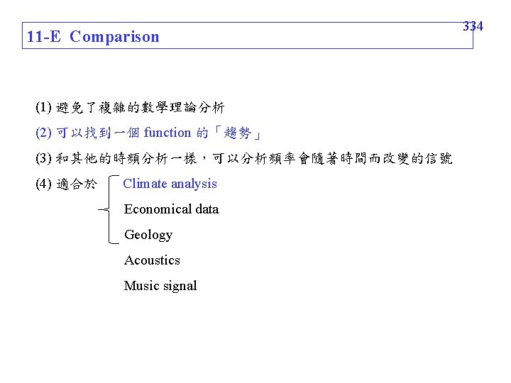
335 Conclusion 當信號含有「趨勢」 或是由少數幾個 sinusoid functions 所組合而成，而且這些sinusoid functions 的 amplitudes 相差懸殊時，可以用 HHT 來分析

附錄十一 Interpolation and the B-Spline Suppose that the sampling points are t 1, t 2, t 3, …, t. N and we have known the values of x(t) at these sampling points. There are several ways for interpolation. (1) The simplest way: Using the straight lines (i. e. , linear interpolation) t 1 t 2 t 3 t 4 336

337 (2) Lagrange interpolation 指的是連乘符號， (3) Polynomial interpolation solve a 1, a 2, a 3, ……, a. N-1 from

338 (4) Lowpass Filter Interpolation 適用於 sampling interval 為固定的情形 tn+1 tn = t for all n discrete time x(tn) Fourier transform X 1(f) lowpass mask X (f) inverse discrete time Fourier transform x(t)

339 (5) B-Spline Interpolation B-spline 簡稱為 spline for tn < tn+1 otherwise m = 1: linear B-spline m = 2: quadratic B-spline m = 3: cubic B-spline (通常使用) are continuous

In Matlab，the command“spline” can be used for spline interpolation (Note： In the command, the cubic B-spline is used) Example: Generating a sine-like spline curve and samples it over a finer mesh: x = 0: 1: 10; % original sampling points y = sin(x); xx = 0: 0. 1: 10; % new sampling points yy = spline(x, y, xx); plot(x, y, 'o', xx, yy) 340