Workshop has been scheduled for Jan 2 3

Workshop has been scheduled for Jan 2 (3 pm-6 pm) Jan 3 (8 am-6 pm) Shown in the current Aerospace America 1

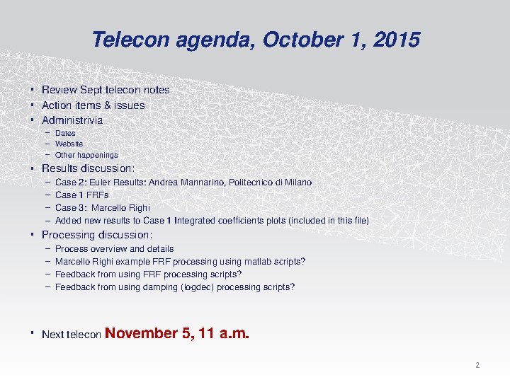
Telecon agenda, October 1, 2015 • Review Sept telecon notes • Action items & issues • Administrivia – Dates – Website – Other happenings • Results discussion: – – Case 2: Euler Results: Andrea Mannarino, Politecnico di Milano Case 1 FRFs Case 3: Marcello Righi Added new results to Case 1 Integrated coefficients plots (included in this file) • Processing discussion: – – Process overview and details Marcello Righi example FRF processing using matlab scripts? Feedback from using FRF processing scripts? Feedback from using damping (logdec) processing scripts? • Next telecon November 5, 11 a. m. 2

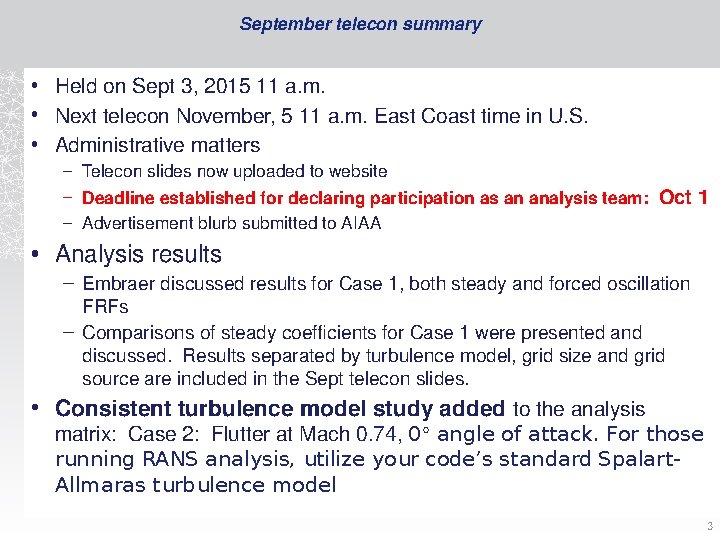
September telecon summary • Held on Sept 3, 2015 11 a. m. • Next telecon November, 5 11 a. m. East Coast time in U. S. • Administrative matters – Telecon slides now uploaded to website – Deadline established for declaring participation as an analysis team: Oct 1 – Advertisement blurb submitted to AIAA • Analysis results – Embraer discussed results for Case 1, both steady and forced oscillation FRFs – Comparisons of steady coefficients for Case 1 were presented and discussed. Results separated by turbulence model, grid size and grid source are included in the Sept telecon slides. • Consistent turbulence model study added to the analysis matrix: Case 2: Flutter at Mach 0. 74, 0° angle of attack. For those running RANS analysis, utilize your code’s standard Spalart. Allmaras turbulence model 3

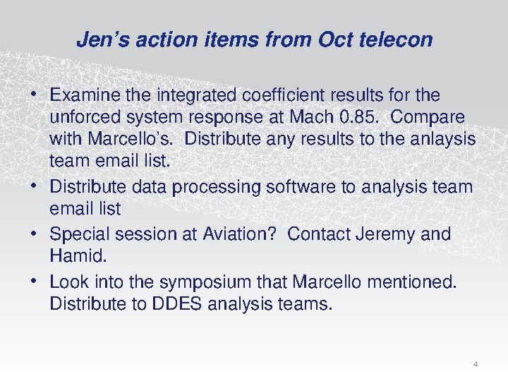
Jen’s action items from Oct telecon • Examine the integrated coefficient results for the unforced system response at Mach 0. 85. Compare with Marcello’s. Distribute any results to the anlaysis team email list. • Distribute data processing software to analysis team email list • Special session at Aviation? Contact Jeremy and Hamid. • Look into the symposium that Marcello mentioned. Distribute to DDES analysis teams. 4

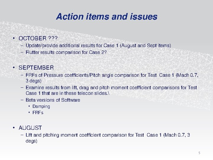
Action items and issues • OCTOBER ? ? ? – Update/provide additional results for Case 1 (August and Sept items) – Flutter results comparison for Case 2? • SEPTEMBER – FRFs of Pressure coefficients/Pitch angle comparison for Test Case 1 (Mach 0. 7, 3 degs) – Examine results from lift, drag and pitch moment coefficient comparisons for Test Case 1 that are in these telecon slides. – Beta versions of Software • Damping • FRFs • AUGUST – Lift and pitching moment coefficient comparison for Test Case 1 (Mach 0. 7, 3 degs) 5

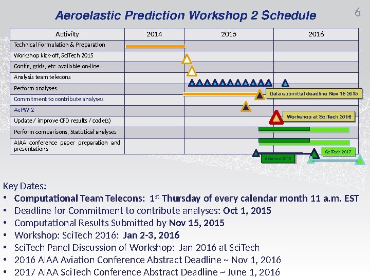
6 Aeroelastic Prediction Workshop 2 Schedule Activity 2014 2015 2016 Technical Formulation & Preparation Workshop kick-off, Sci. Tech 2015 Config, grids, etc. available on-line Analysis team telecons Perform analyses. Commitment to contribute analyses Data submittal deadline Nov 15 15 2015 Ae. PW-2 Update / improve CFD results / code(s) Workshop at at Sci. Tech 2016 Perform comparisons, Statistical analyses AIAA conference paper preparation and presentations Sci. Tech 2017 Aviation 2016 Key Dates: • Computational Team Telecons: 1 st Thursday of every calendar month 11 a. m. EST • Deadline for Commitment to contribute analyses: Oct 1, 2015 • Computational Results Submitted by Nov 15, 2015 • Workshop: Sci. Tech 2016: Jan 2 -3, 2016 • Sci. Tech Panel Discussion of Workshop: Jan 2016 at Sci. Tech • 2016 AIAA Aviation Conference Abstract Deadline ~ Nov 1, 2016 • 2017 AIAA Sci. Tech Conference Abstract Deadline ~ June 1, 2016

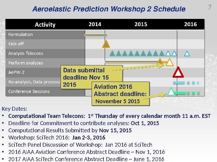
Aeroelastic Prediction Workshop 2 Schedule 7 Data submittal deadline Nov 15 15 2015 Aviation 2016 Abstract deadline: November 55 2015 Key Dates: • Computational Team Telecons: 1 st Thursday of every calendar month 11 a. m. EST • Deadline for Commitment to contribute analyses: Oct 1, 2015 • Computational Results Submitted by Nov 15, 2015 • Workshop: Sci. Tech 2016: Jan 2 -3, 2016 • Sci. Tech Panel Discussion of Workshop: Jan 2016 at Sci. Tech • 2016 AIAA Aviation Conference Abstract Deadline ~ Nov 1, 2016 • 2017 AIAA Sci. Tech Conference Abstract Deadline ~ June 1, 2016

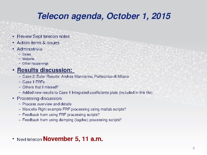
Telecon agenda, October 1, 2015 • Review Sept telecon notes • Action items & issues • Administrivia – Dates – Website – Other happenings • Results discussion: – – Case 2: Euler Results: Andrea Mannarino, Politecnico di Milano Case 1 FRFs Others that I missed? Added new results to Case 1 Integrated coefficients plots (included in this file) • Processing discussion: – – Process overview and details Marcello Righi example FRF processing using matlab scripts? Feedback from using FRF processing scripts? Feedback from using damping (logdec) processing scripts? • Next telecon November 5, 11 a. m. 8

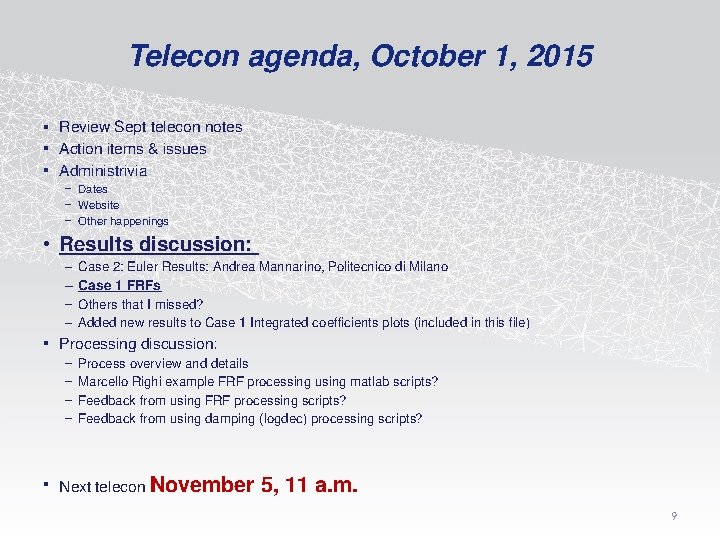
Telecon agenda, October 1, 2015 • Review Sept telecon notes • Action items & issues • Administrivia – Dates – Website – Other happenings • Results discussion: – – Case 2: Euler Results: Andrea Mannarino, Politecnico di Milano Case 1 FRFs Others that I missed? Added new results to Case 1 Integrated coefficients plots (included in this file) • Processing discussion: – – Process overview and details Marcello Righi example FRF processing using matlab scripts? Feedback from using FRF processing scripts? Feedback from using damping (logdec) processing scripts? • Next telecon November 5, 11 a. m. 9

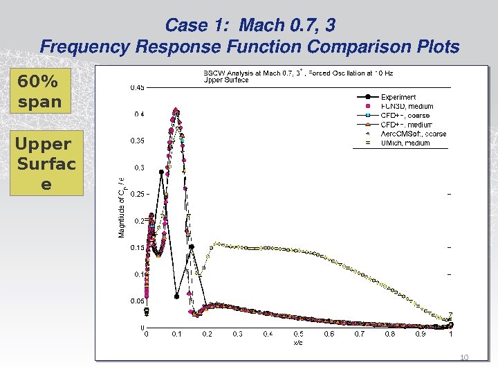
Case 1: Mach 0. 7, 3 Frequency Response Function Comparison Plots 60% span Upper Surfac e 10

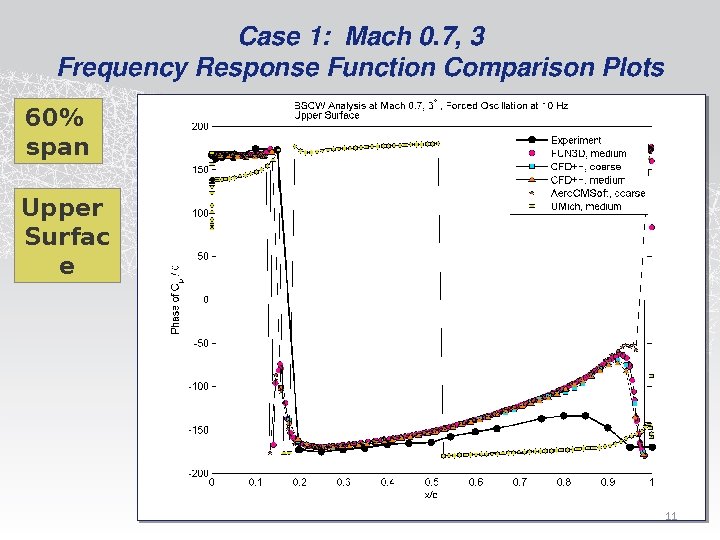
Case 1: Mach 0. 7, 3 Frequency Response Function Comparison Plots 60% span Upper Surfac e 11

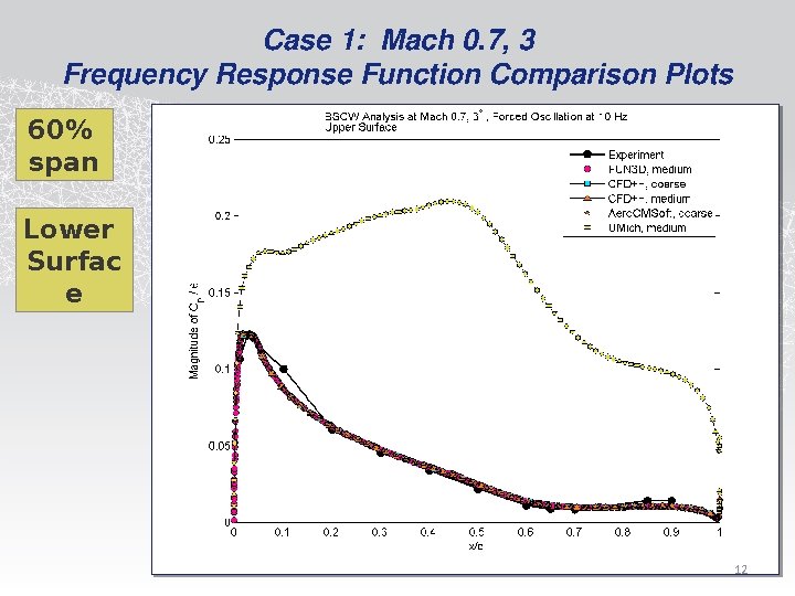
Case 1: Mach 0. 7, 3 Frequency Response Function Comparison Plots 60% span Lower Surfac e 12

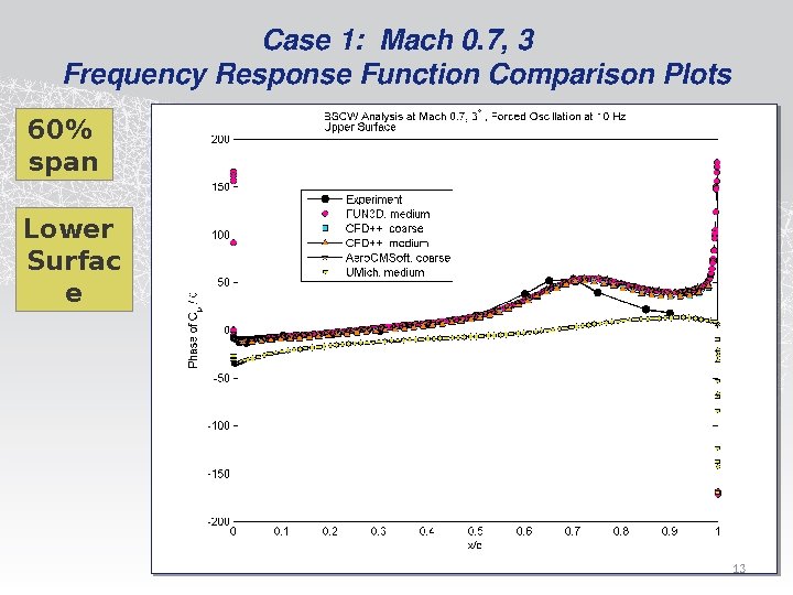
Case 1: Mach 0. 7, 3 Frequency Response Function Comparison Plots 60% span Lower Surfac e 13

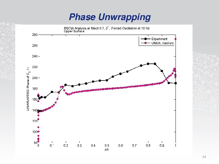
Phase Unwrapping 14

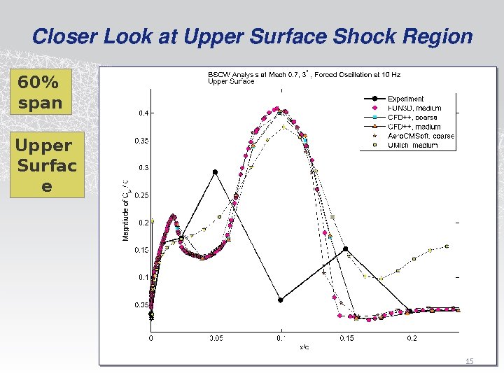
Closer Look at Upper Surface Shock Region 60% span Upper Surfac e 15

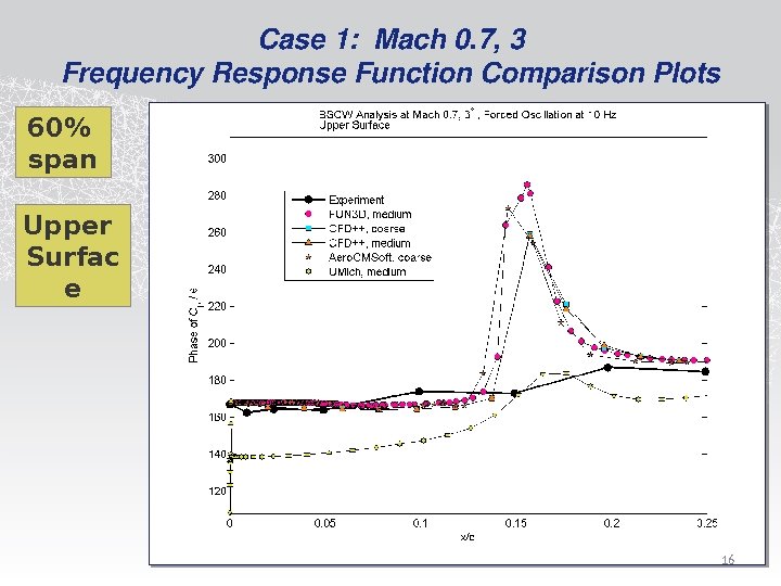
Case 1: Mach 0. 7, 3 Frequency Response Function Comparison Plots 60% span Upper Surfac e 16

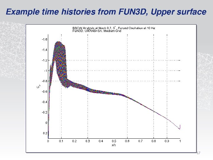
Example time histories from FUN 3 D, Upper surface 17

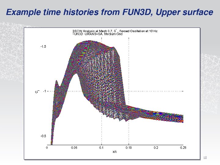
Example time histories from FUN 3 D, Upper surface 18

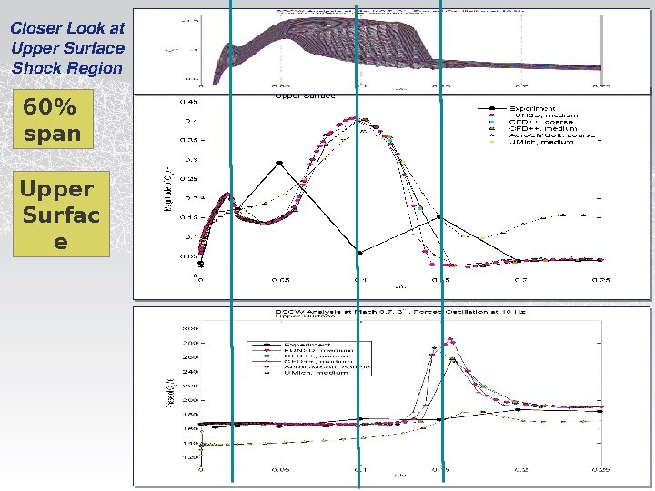
Closer Look at Upper Surface Shock Region 60% span Upper Surfac e 19

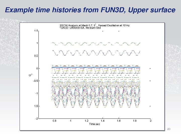
Example time histories from FUN 3 D, Upper surface 20

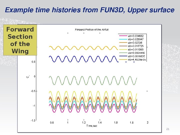
Example time histories from FUN 3 D, Upper surface Forward Section of the Wing 21

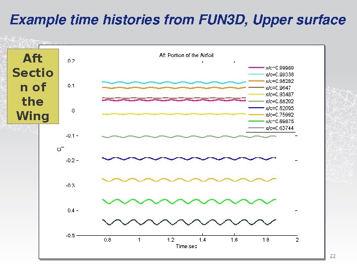
Example time histories from FUN 3 D, Upper surface Aft Sectio n of the Wing 22

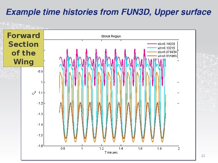
Example time histories from FUN 3 D, Upper surface Forward Section of the Wing 23

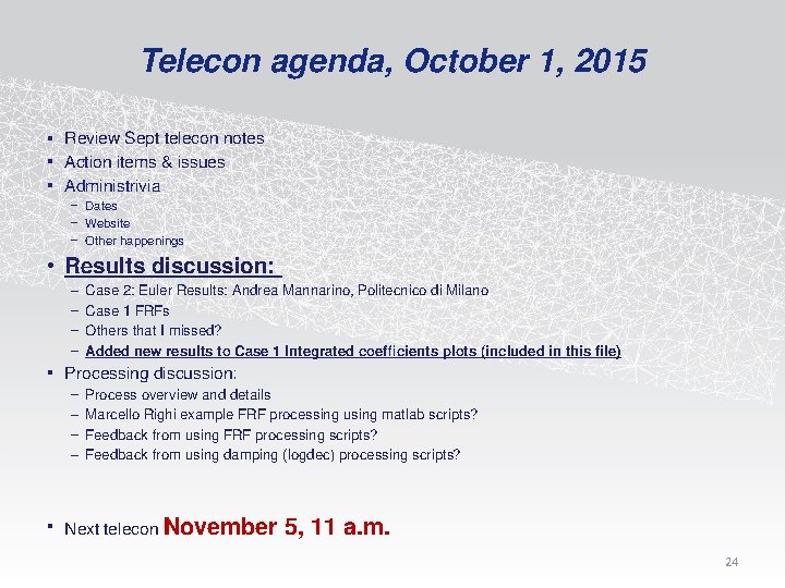
Telecon agenda, October 1, 2015 • Review Sept telecon notes • Action items & issues • Administrivia – Dates – Website – Other happenings • Results discussion: – – Case 2: Euler Results: Andrea Mannarino, Politecnico di Milano Case 1 FRFs Others that I missed? Added new results to Case 1 Integrated coefficients plots (included in this file) • Processing discussion: – – Process overview and details Marcello Righi example FRF processing using matlab scripts? Feedback from using FRF processing scripts? Feedback from using damping (logdec) processing scripts? • Next telecon November 5, 11 a. m. 24

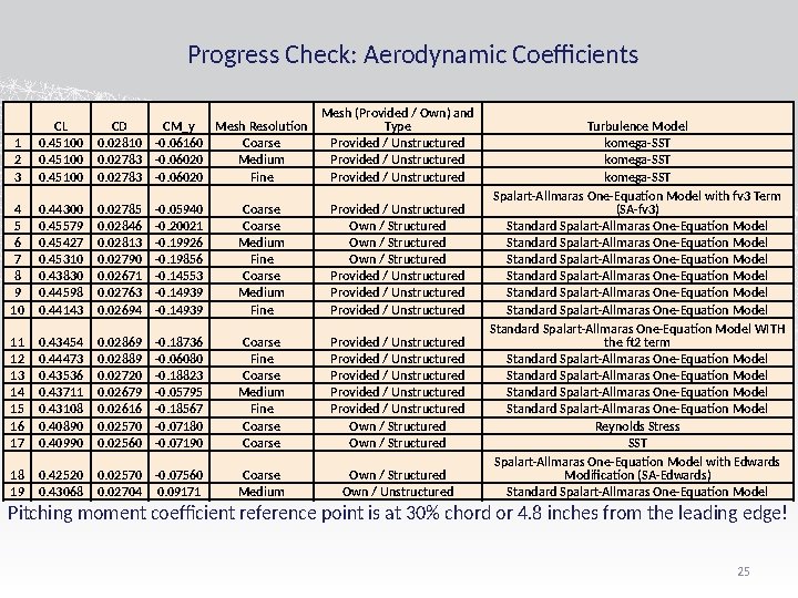
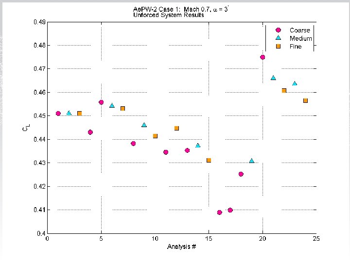
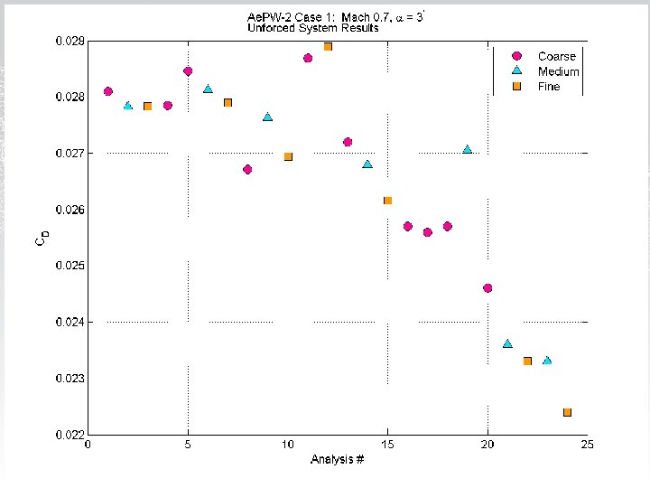
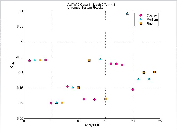
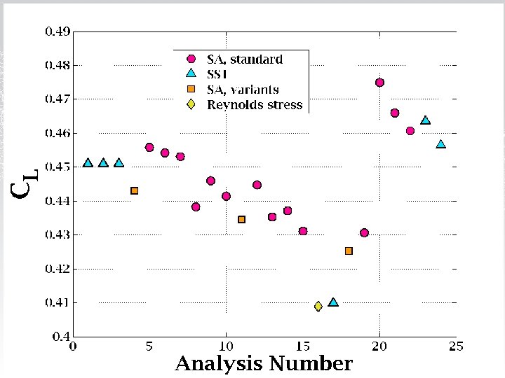
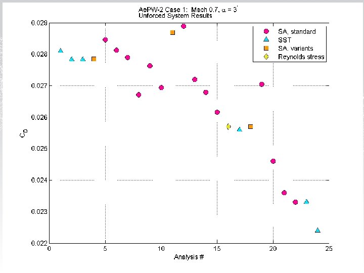
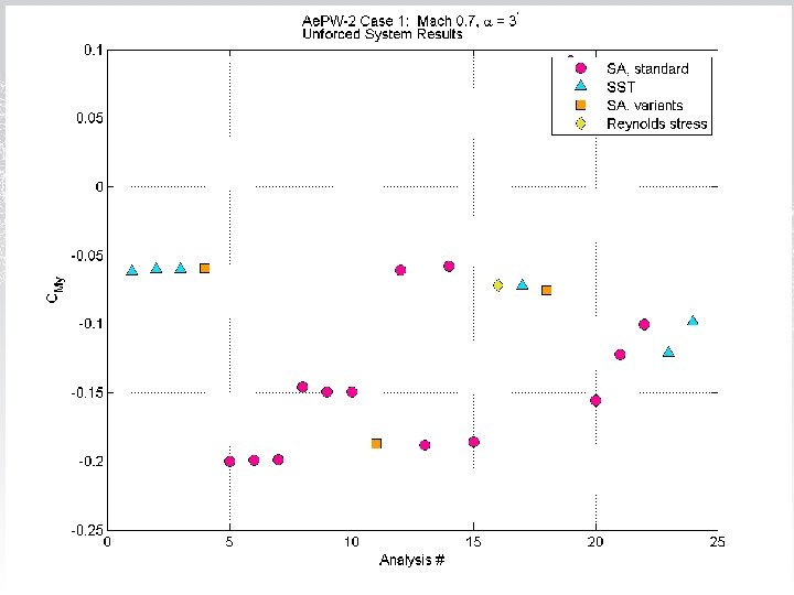
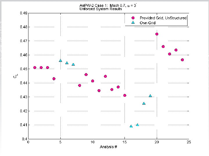
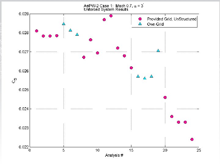
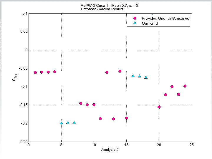
Progress Check: Aerodynamic Coefficients Mesh (Provided / Own) and Type Provided / Unstructured 1 2 3 CL 0. 45100 CD 0. 02810 0. 02783 CM_y Mesh Resolution -0. 06160 Coarse -0. 06020 Medium -0. 06020 Fine 4 5 6 7 8 9 10 0. 44300 0. 45579 0. 45427 0. 45310 0. 43830 0. 44598 0. 44143 0. 02785 0. 02846 0. 02813 0. 02790 0. 02671 0. 02763 0. 02694 -0. 05940 -0. 20021 -0. 19926 -0. 19856 -0. 14553 -0. 14939 Coarse Medium Fine Provided / Unstructured Own / Structured Provided / Unstructured 11 12 13 14 15 16 17 0. 43454 0. 44473 0. 43536 0. 43711 0. 43108 0. 40890 0. 40990 0. 02869 0. 02889 0. 02720 0. 02679 0. 02616 0. 02570 0. 02560 -0. 18736 -0. 06080 -0. 18823 -0. 05795 -0. 18567 -0. 07180 -0. 07190 Coarse Fine Coarse Medium Fine Coarse Provided / Unstructured Provided / Unstructured Own / Structured 18 19 0. 42520 0. 43068 0. 02570 0. 02704 -0. 07560 0. 09171 Coarse Medium Own / Structured Own / Unstructured Turbulence Model komega-SST Spalart-Allmaras One-Equation Model with fv 3 Term (SA-fv 3) Standard Spalart-Allmaras One-Equation Model Standard Spalart-Allmaras One-Equation Model WITH the ft 2 term Standard Spalart-Allmaras One-Equation Model Reynolds Stress SST Spalart-Allmaras One-Equation Model with Edwards Modification (SA-Edwards) Standard Spalart-Allmaras One-Equation Model Pitching moment coefficient reference point is at 30% chord or 4. 8 inches from the leading edge! 25

26

27

28

29

30

31

32

33

34

Telecon agenda, October 1, 2015 • Review Sept telecon notes • Action items & issues • Administrivia – Dates – Website – Other happenings • Results discussion: – – Case 2: Euler Results: Andrea Mannarino, Politecnico di Milano Case 1 FRFs Others that I missed? Added new results to Case 1 Integrated coefficients plots (included in this file) • Processing discussion: – – Process overview and details Marcello Righi example FRF processing using matlab scripts? Feedback from using FRF processing scripts? Feedback from using damping (logdec) processing scripts? • Next telecon November 5, 11 a. m. 35

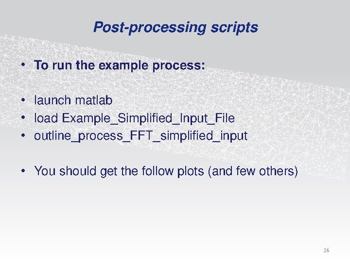
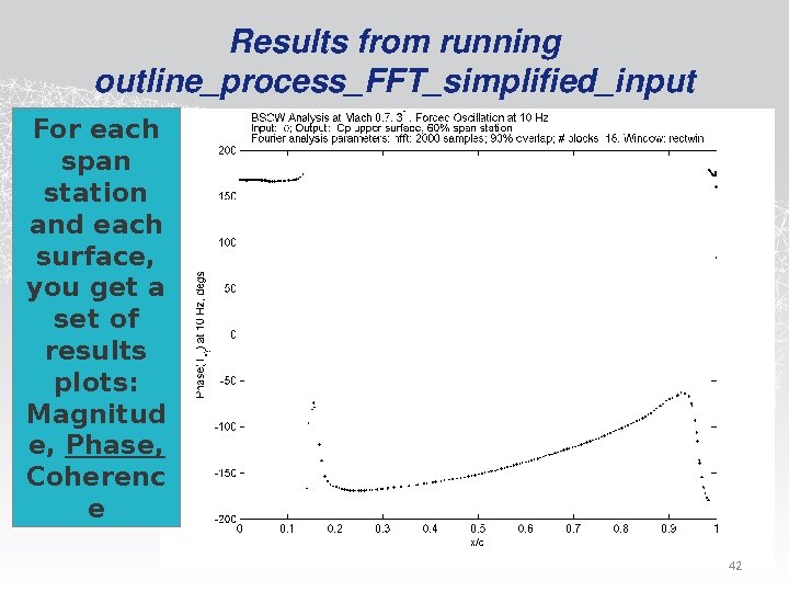
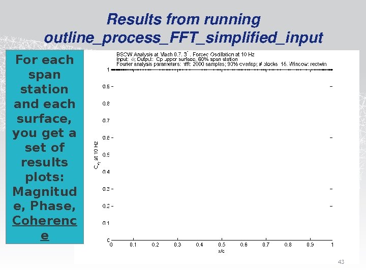
Post-processing scripts • To run the example process: • launch matlab • load Example_Simplified_Input_File • outline_process_FFT_simplified_input • You should get the follow plots (and few others) 36

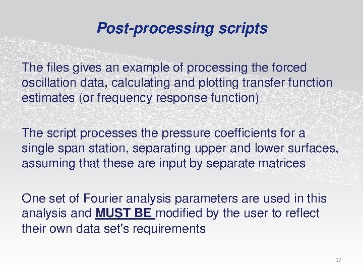
Post-processing scripts The files gives an example of processing the forced oscillation data, calculating and plotting transfer function estimates (or frequency response function) The script processes the pressure coefficients for a single span station, separating upper and lower surfaces, assuming that these are input by separate matrices One set of Fourier analysis parameters are used in this analysis and MUST BE modified by the user to reflect their own data set's requirements 37

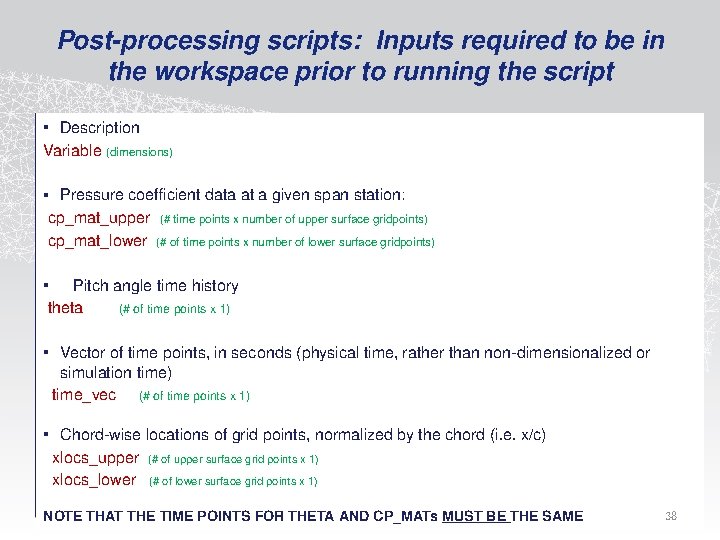
Post-processing scripts: Inputs required to be in the workspace prior to running the script • Description Variable (dimensions) • Pressure coefficient data at a given span station: cp_mat_upper (# time points x number of upper surface gridpoints) cp_mat_lower (# of time points x number of lower surface gridpoints) • Pitch angle time history theta (# of time points x 1) • Vector of time points, in seconds (physical time, rather than non-dimensionalized or simulation time) time_vec (# of time points x 1) • Chord-wise locations of grid points, normalized by the chord (i. e. x/c) xlocs_upper (# of upper surface grid points x 1) xlocs_lower (# of lower surface grid points x 1) NOTE THAT THE TIME POINTS FOR THETA AND CP_MATs MUST BE THE SAME 38

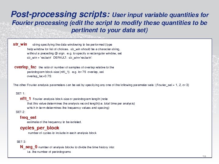
Post-processing scripts: User input variable quantities for Fourier processing (edit the script to modify these quantities to be pertinent to your data set) str_win string specifying the data windowing to be performed (type help window for list of choices. str_win should be a character string, without a preceding @ sign. e. g. to specify a rectangular window, set str_win = 'rectwin' DEFAULT: str_win='rectwin'; overlap_fac the ratio of number of samples of overlap relative to the periodogram block size (nfft_1). e. g. for 75 overlap, set overlap_fac=0. 75; The other Fourier analysis parameters can be set by specifying any one of the following parameter sets: (Fourier_set = 1, 2, or 3) SET 1: nfft_1 Fourier analysis block size or periodogram length (note that this value determines the analysis record length(i. e. total time per analysis) which in term determines the frequency values and spacing) SET 2: freq_est estimate of the frequency to be isolated. cycles_per_block number of cycles to include in each analysis block SET 3: N_seg_0 number of analysis blocks to divide the time history into; i. e. the number of periodograms 39

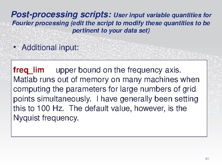
Post-processing scripts: User input variable quantities for Fourier processing (edit the script to modify these quantities to be pertinent to your data set) • Additional input: freq_lim upper bound on the frequency axis. Matlab runs out of memory on many machines when computing the parameters for large numbers of grid points simultaneously. I have generally been setting this to 100 Hz. The default value, however, is the Nyquist frequency. 40

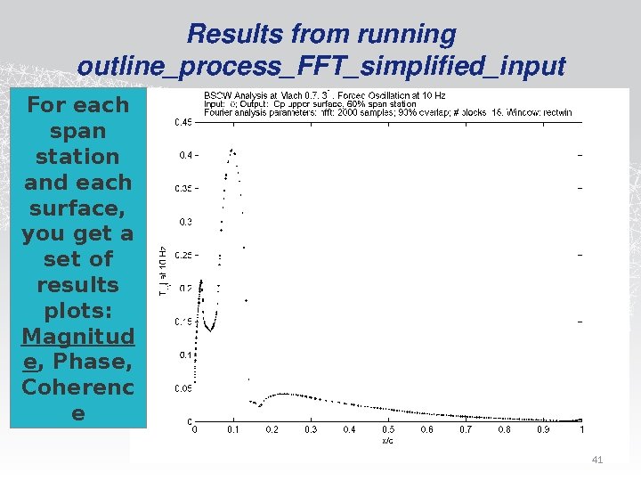
Results from running outline_process_FFT_simplified_input For each span station and each surface, you get a set of results plots: Magnitud e, Phase, Coherenc e 41

Results from running outline_process_FFT_simplified_input For each span station and each surface, you get a set of results plots: Magnitud e, Phase, Coherenc e 42

Results from running outline_process_FFT_simplified_input For each span station and each surface, you get a set of results plots: Magnitud e, Phase, Coherenc e 43

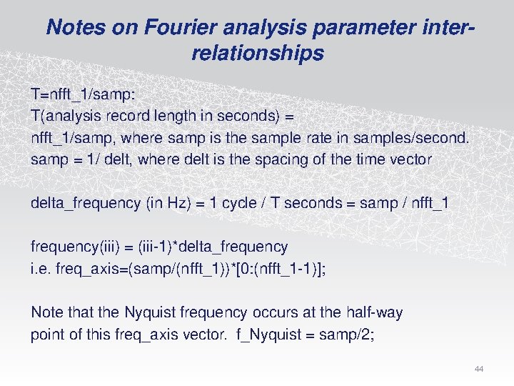
Notes on Fourier analysis parameter interrelationships T=nfft_1/samp: T(analysis record length in seconds) = nfft_1/samp, where samp is the sample rate in samples/second. samp = 1/ delt, where delt is the spacing of the time vector delta_frequency (in Hz) = 1 cycle / T seconds = samp / nfft_1 frequency(iii) = (iii-1)*delta_frequency i. e. freq_axis=(samp/(nfft_1))*[0: (nfft_1 -1)]; Note that the Nyquist frequency occurs at the half-way point of this freq_axis vector. f_Nyquist = samp/2; 44

Scripts included in the beta release • read_tecplot_file. m (read point-stacked tecplot file into matlab data structure db_tec. Variables are stored as fields of that data structure) • outline_process_FFT_simplified_input • periodogram_mimo_jh (multi-input multi-output cross-spectral density function calculation) • periodogram_jh (for computing 1 cross-spectral density function at a time) • correct_PSD_for_window (called by periodogram program) • overlap_func_approx_nfft • fmult • fdiv • fmash • Example_Simplified_Input_File. mat 45

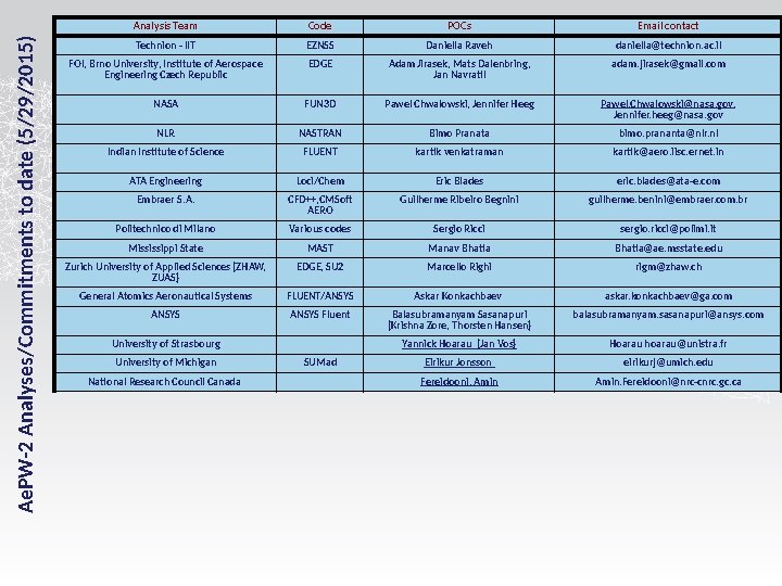
Ae. PW-2 Analyses/Commitments to date (5/29/2015) Analysis Team Code POCs Email contact Technion - IIT EZNSS Daniella Raveh daniella@technion. ac. il FOI, Brno University, Institute of Aerospace Engineering Czech Republic EDGE Adam Jirasek, Mats Dalenbring, Jan Navratil adam. jirasek@gmail. com NASA FUN 3 D Pawel Chwalowski, Jennifer Heeg Pawel. Chwalowski@nasa. gov, Jennifer. heeg@nasa. gov NLR NASTRAN Bimo Pranata bimo. prananta@nlr. nl Indian Institute of Science FLUENT kartik venkatraman kartik@aero. iisc. ernet. in ATA Engineering Loci/Chem Eric Blades eric. blades@ata-e. com Embraer S. A. CFD++, CMSoft AERO Guilherme Ribeiro Begnini guilherme. benini@embraer. com. br Politechnico di Milano Various codes Sergio Ricci sergio. ricci@polimi. it Mississippi State MAST Manav Bhatia@ae. msstate. edu Zurich University of Applied Sciences (ZHAW, ZUAS) EDGE, SU 2 Marcello Righi rigm@zhaw. ch General Atomics Aeronautical Systems FLUENT/ANSYS Askar Konkachbaev askar. konkachbaev@ga. com ANSYS Fluent Balasubramanyam Sasanapuri (Krishna Zore, Thorsten Hansen) balasubramanyam. sasanapuri@ansys. com Yannick Hoarau (Jan Vos) Hoarau hoarau@unistra. fr Eirikur Jonsson eirikurj@umich. edu Fereidooni, Amin. Fereidooni@nrc-cnrc. gc. ca University of Strasbourg University of Michigan National Research Council Canada SUMad

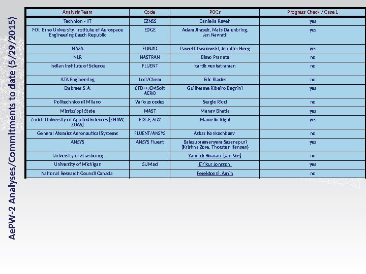
Ae. PW-2 Analyses/Commitments to date (5/29/2015) Analysis Team Code POCs Progress Check / Case 1 Technion - IIT EZNSS Daniella Raveh yes FOI, Brno University, Institute of Aerospace Engineering Czech Republic EDGE Adam Jirasek, Mats Dalenbring, Jan Navratil yes NASA FUN 3 D Pawel Chwalowski, Jennifer Heeg yes NLR NASTRAN Bimo Pranata no Indian Institute of Science FLUENT kartik venkatraman no ATA Engineering Loci/Chem Eric Blades no Embraer S. A. CFD++, CMSoft AERO Guilherme Ribeiro Begnini yes Politechnico di Milano Various codes Sergio Ricci no Mississippi State MAST Manav Bhatia yes Zurich University of Applied Sciences (ZHAW, ZUAS) EDGE, SU 2 Marcello Righi yes General Atomics Aeronautical Systems FLUENT/ANSYS Askar Konkachbaev no ANSYS Fluent Balasubramanyam Sasanapuri (Krishna Zore, Thorsten Hansen) yes Yannick Hoarau (Jan Vos) no Eirikur Jonsson yes Fereidooni, Amin no University of Strasbourg University of Michigan National Research Council Canada SUMad

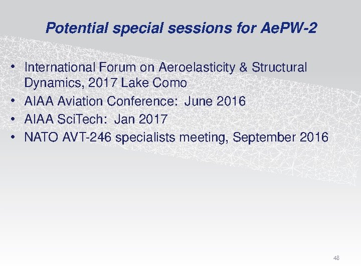
Potential special sessions for Ae. PW-2 • International Forum on Aeroelasticity & Structural Dynamics, 2017 Lake Como • AIAA Aviation Conference: June 2016 • AIAA Sci. Tech: Jan 2017 • NATO AVT-246 specialists meeting, September 2016 48

• Preliminary Meeting Announcement • • CALL FOR PAPERS • for the • AVT-246 Specialists’ Meeting (RSM) • • on Progress and Challenges in Validation Testing for Computational Fluid Dynamics • • Organized by the Members of the APPLIED VEHICLE TECHNOLOGY PANEL (AVT) AVT-246 – • and to be held in Zaragoza, Spain 26 -28 September 2016 Contributions and participation are invited from NATO Nations, Australia and Sweden only • Final Deadline for submission of abstracts is 1 October 2015 49

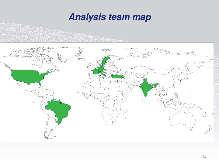
Analysis team map 50

Telecon agenda, September 3, 2015 • Review July/August telecon notes • Action items & issues • Administrivia – – Dates Website AIAA coordination Other happenings • Results discussion: Embraer S. A. • Next telecon: October 1, 11 am 51

Frequency response function estimates using fourier analysis • references: • Oppenheim & Shafer, Discrete-time signal processing • Jay Hardin, NASA RP-1145, Introduction to time series analysis • Bendat & Pierson, Engineering applications of correlation and spectral analysis 52

Frequency response functions (FRFs) magnitude calculation example Magnitude of of FRF, Cp/q FRFy , x ( f ) CSD y , x ( f ) PSDx ( f ) Here, x = pitch angle y = Cp • 1 FRF for each pressure transducer or grid point Frequency, Hz Pressure / excitation: At frequencies where there is no excitation, the calculation is dividing by 0’ish numbers, making the FRF a large amplitude noisy response

Frequency response functions (FRFs) magnitude calculation example Magnitude of of FRF, Cp/q FRFy , x ( f ) CSD y , x ( f ) PSDx ( f ) Here, x = pitch angle y = Cp • 1 FRF for each pressure transducer or grid point • Examine values only at the excitation frequency Frequency, Hz Excitation frequency , in this example, ~80 Hz

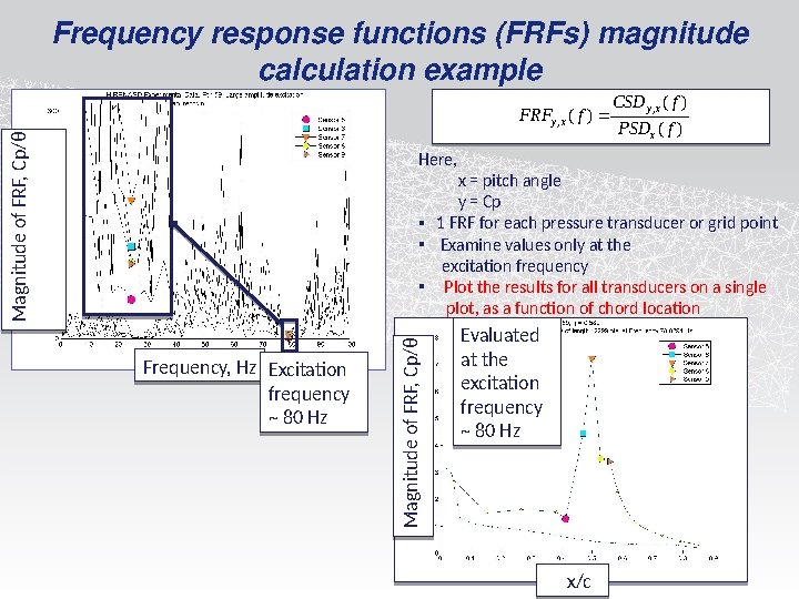
Frequency response functions (FRFs) magnitude calculation example Magnitude of of FRF, Cp/q FRFy , x ( f ) CSD y , x ( f ) PSDx ( f ) Here, Frequency, Hz Excitation frequency ~ 80 Hz Magnitude of of FRF, Cp/q x = pitch angle y = Cp • 1 FRF for each pressure transducer or grid point • Examine values only at the excitation frequency • Plot the results for all transducers on a single plot, as a function of chord location Evaluated at the excitation frequency ~ 80 Hz x/c

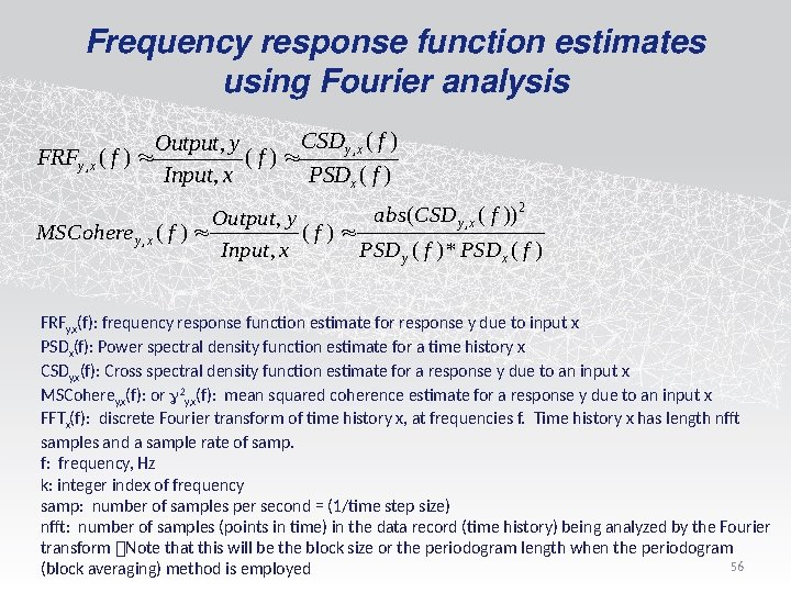
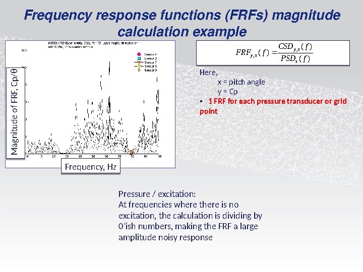
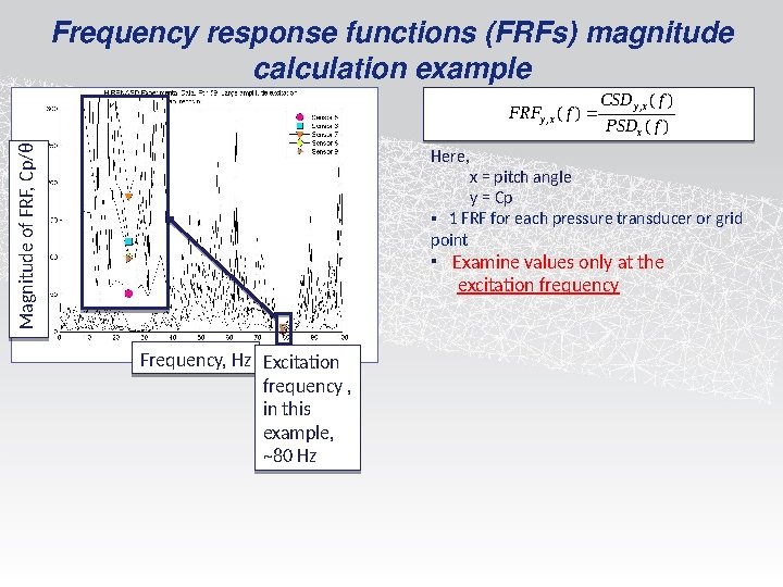
Frequency response function estimates using Fourier analysis CSDy , x ( f ) Output, y FRFy , x ( f ) (f) Input, x PSDx ( f ) abs(CSD y , x ( f )) 2 Output , y MSCohere y , x ( f ) (f) Input, x PSD y ( f ) * PSDx ( f ) FRFy, x(f): frequency response function estimate for response y due to input x PSDx(f): Power spectral density function estimate for a time history x CSDy, x(f): Cross spectral density function estimate for a response y due to an input x MSCoherey, x(f): or g 2 y, x(f): mean squared coherence estimate for a response y due to an input x FFTx(f): discrete Fourier transform of time history x, at frequencies f. Time history x has length nfft samples and a sample rate of samp. f: frequency, Hz k: integer index of frequency samp: number of samples per second = (1/time step size) nfft: number of samples (points in time) in the data record (time history) being analyzed by the Fourier transform Note that this will be the block size or the periodogram length when the periodogram 56 (block averaging) method is employed

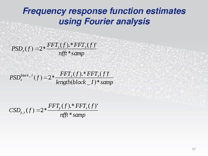
Frequency response function estimates using Fourier analysis PSDx ( f ) 2 * FFTx ( f )' nfft * samp PSDxblock _ I ( f ) 2 * CSD y , x ( f ) 2 * FFTx ( f )' length(block _ I ) * samp FFTy ( f ). * FFTx ( f )' nfft * samp 57

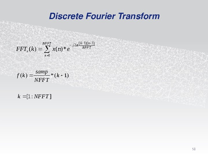
Discrete Fourier Transform NFFT FFTx (k ) x(n) * e j 2 ( k 1)( n 1) NFFT n 1 f (k ) samp * (k 1) NFFT k [1 : NFFT ] 58

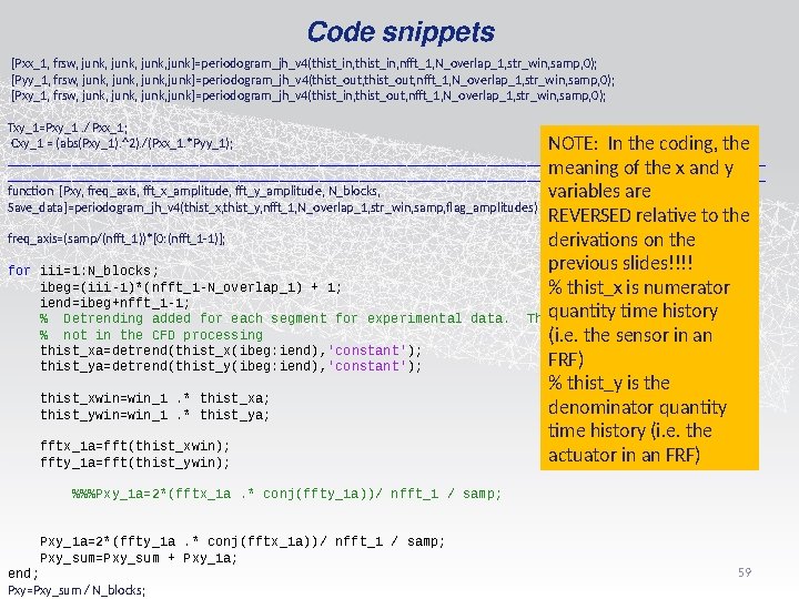
Code snippets [Pxx_1, frsw, junk, junk]=periodogram_jh_v 4(thist_in, nfft_1, N_overlap_1, str_win, samp, 0); [Pyy_1, frsw, junk, junk]=periodogram_jh_v 4(thist_out, nfft_1, N_overlap_1, str_win, samp, 0); [Pxy_1, frsw, junk, junk]=periodogram_jh_v 4(thist_in, thist_out, nfft_1, N_overlap_1, str_win, samp, 0); Txy_1=Pxy_1. / Pxx_1; Cxy_1 = (abs(Pxy_1). ^2). /(Pxx_1. *Pyy_1); NOTE: In the coding, the ________________________________________________ meaning of the x and y ________________________________________________ function [Pxy, freq_axis, fft_x_amplitude, fft_y_amplitude, N_blocks, variables are Save_data]=periodogram_jh_v 4(thist_x, thist_y, nfft_1, N_overlap_1, str_win, samp, flag_amplitudes) freq_axis=(samp/(nfft_1))*[0: (nfft_1 -1)]; for iii=1: N_blocks; ibeg=(iii-1)*(nfft_1 -N_overlap_1) + 1; iend=ibeg+nfft_1 -1; % Detrending added for each segment for experimental data. % not in the CFD processing thist_xa=detrend(thist_x(ibeg: iend), 'constant'); thist_ya=detrend(thist_y(ibeg: iend), 'constant'); thist_xwin=win_1. * thist_xa; thist_ywin=win_1. * thist_ya; fftx_1 a=fft(thist_xwin); ffty_1 a=fft(thist_ywin); REVERSED relative to the derivations on the previous slides!!!! % thist_x is numerator quantity time history This is (i. e. the sensor in an FRF) % thist_y is the denominator quantity time history (i. e. the actuator in an FRF) %%%Pxy_1 a=2*(fftx_1 a. * conj(ffty_1 a))/ nfft_1 / samp; Pxy_1 a=2*(ffty_1 a. * conj(fftx_1 a))/ nfft_1 / samp; Pxy_sum=Pxy_sum + Pxy_1 a; end; Pxy=Pxy_sum / N_blocks; 59

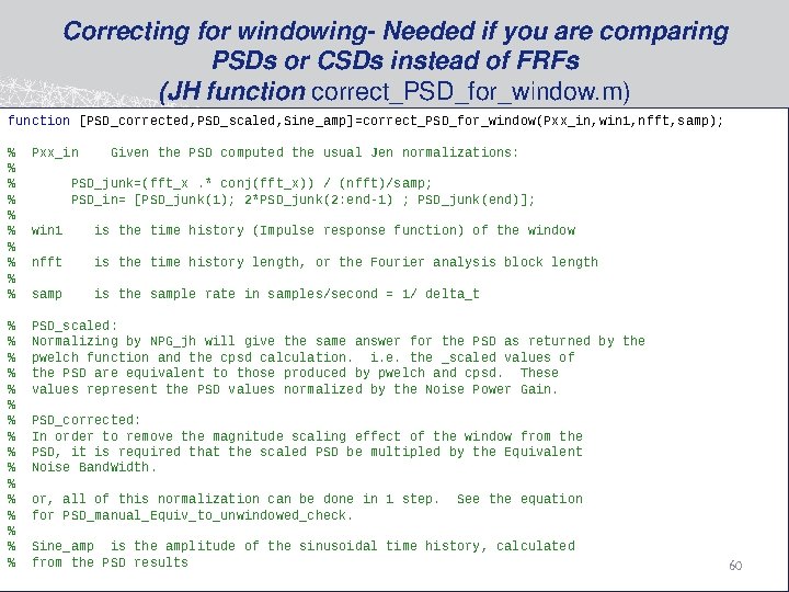
Correcting for windowing- Needed if you are comparing PSDs or CSDs instead of FRFs (JH function correct_PSD_for_window. m) function [PSD_corrected, PSD_scaled, Sine_amp]=correct_PSD_for_window(Pxx_in, win 1, nfft, samp); % % % % % Pxx_in Given the PSD computed the usual Jen normalizations: % % % % PSD_scaled: Normalizing by NPG_jh will give the same answer for the PSD as returned by the pwelch function and the cpsd calculation. i. e. the _scaled values of the PSD are equivalent to those produced by pwelch and cpsd. These values represent the PSD values normalized by the Noise Power Gain. PSD_junk=(fft_x. * conj(fft_x)) / (nfft)/samp; PSD_in= [PSD_junk(1); 2*PSD_junk(2: end-1) ; PSD_junk(end)]; win 1 is the time history (Impulse response function) of the window nfft is the time history length, or the Fourier analysis block length samp is the sample rate in samples/second = 1/ delta_t PSD_corrected: In order to remove the magnitude scaling effect of the window from the PSD, it is required that the scaled PSD be multipled by the Equivalent Noise Band. Width. or, all of this normalization can be done in 1 step. for PSD_manual_Equiv_to_unwindowed_check. See the equation Sine_amp is the amplitude of the sinusoidal time history, calculated from the PSD results 60

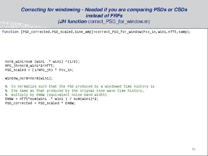
Correcting for windowing - Needed if you are comparing PSDs or CSDs instead of FRFs (JH function correct_PSD_for_window. m) function [PSD_corrected, PSD_scaled, Sine_amp]=correct_PSD_for_window(Pxx_in, win 1, nfft, samp); norm_win 1=sum (win 1. * win 1) ^(1/2); NPG_jh=norm_win 1^2/nfft; PSD_scaled = (1/NPG_jh) * Pxx_in; Window_norm=norm(win 1); % to normalize such that the PSD produced by a windowed time history is % the same as that produced by the orignal sine wave time history, % multiply by ENBW (equivalent noise band width) ENBW = nfft*sum(win 1. * win 1 ) / sum(win 1)^2; PSD_corrected = PSD_scaled * ENBW; 61

Telecon agenda, August 6, 2015 • Review July telecon notes • Action items & issues • Administrivia – – Dates Website AIAA coordination Other happenings • Results discussion • Post processing topics – Frequency response function calculations – Damping calculation (loss factor) • Next telecon Sept 3, 11 a. m. 62

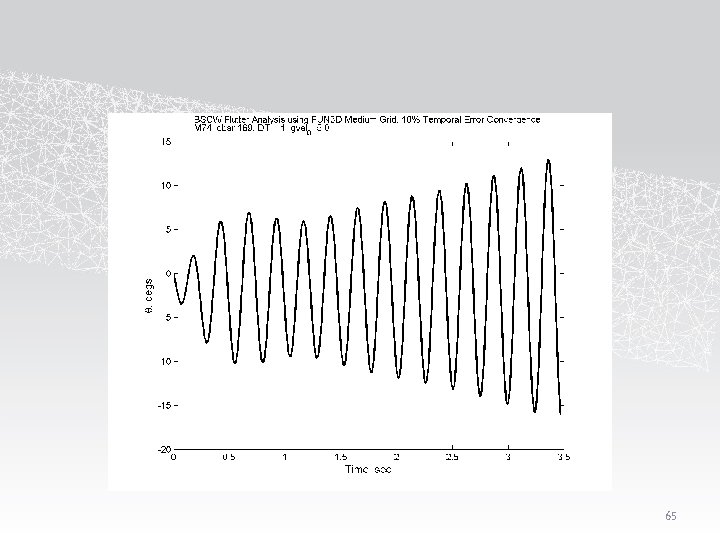
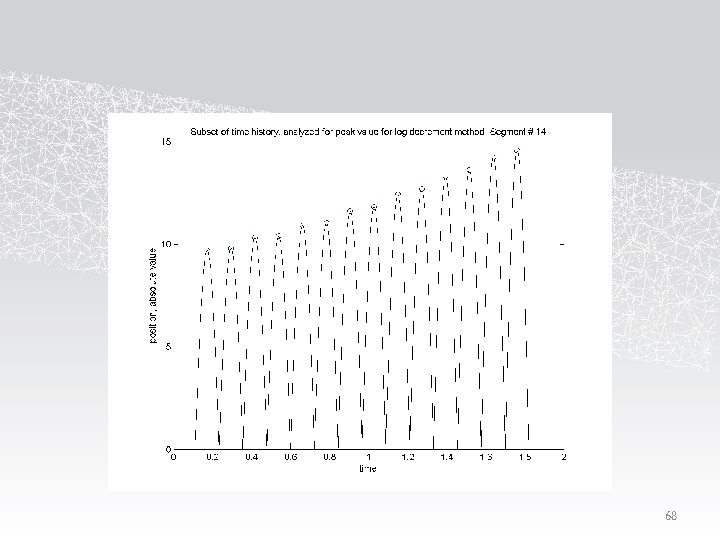
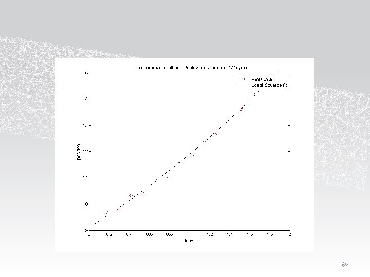
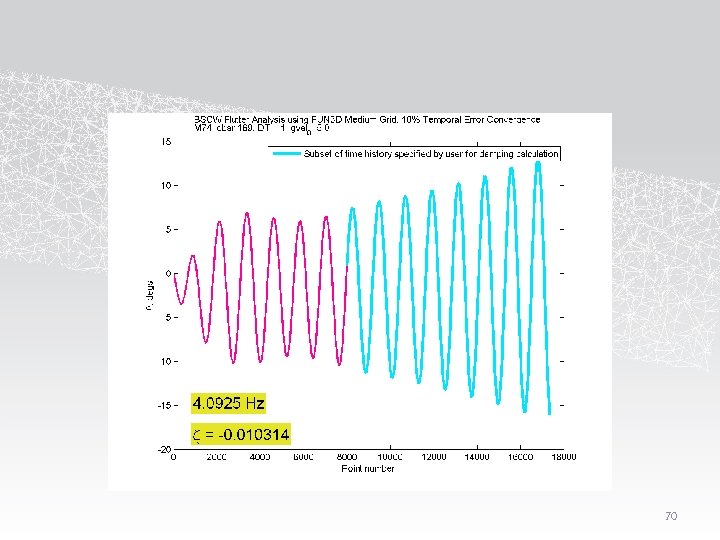
Damping calculation using logarithmic decrement with moving block technique • This isn’t the only method to determine the modal damping. • It is based on the assumption of a single degree of freedom with damped harmonic oscillation. • Damping should ideally be calculated using the pitch angle. • The method can be used on the generalized displacement results, but note that for cases with any significant amount of dynamic pressure, the modes are coupled. They have to be combined to represent a physical quantity. 63

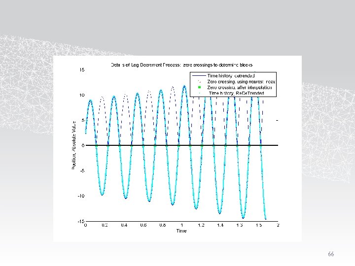
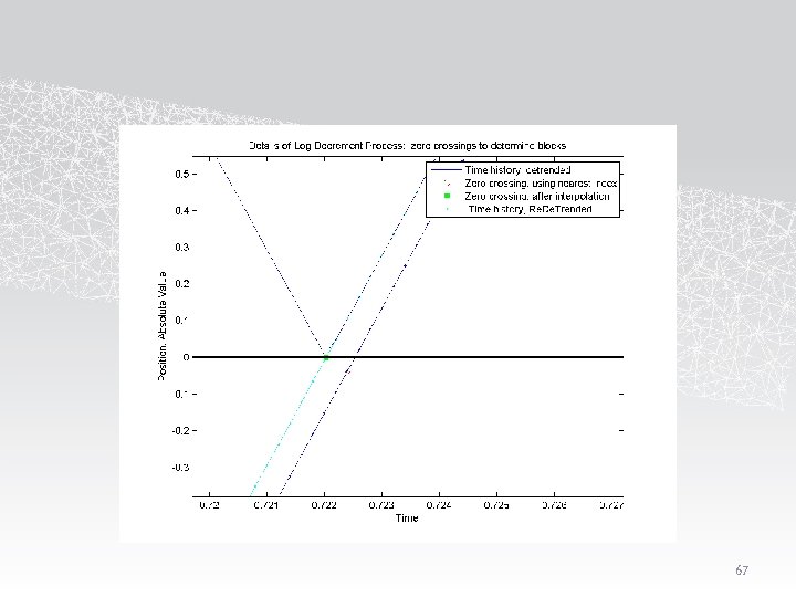
Logarithmic Decrement applied to Ae. PW-2 analysis results: Outline of method • Compute pitch angle • Subset the data by user-interactive data points for beginning and end points • Remove the mean • Determine zero crossings • Interpolate to find improved detrending parameters • Utilize the absolute value of the detrended time history • Take logarithm of peak values for each ½ cycle block • Perform Least squares fit to the data • damping=-1*Linear term coefficient / Mean_freq_rad; 64

65

66

67

68

69

70

General material and prior telecon summaries 71

Updated analysis parameter table 72

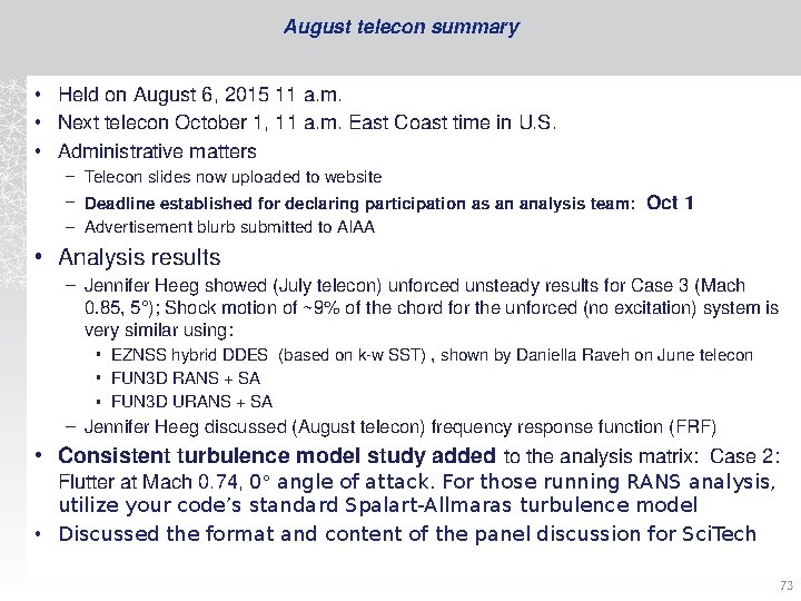
August telecon summary • Held on August 6, 2015 11 a. m. • Next telecon October 1, 11 a. m. East Coast time in U. S. • Administrative matters – Telecon slides now uploaded to website – Deadline established for declaring participation as an analysis team: Oct 1 – Advertisement blurb submitted to AIAA • Analysis results – Jennifer Heeg showed (July telecon) unforced unsteady results for Case 3 (Mach 0. 85, 5°); Shock motion of ~9% of the chord for the unforced (no excitation) system is very similar using: • EZNSS hybrid DDES (based on k-w SST) , shown by Daniella Raveh on June telecon • FUN 3 D RANS + SA • FUN 3 D URANS + SA – Jennifer Heeg discussed (August telecon) frequency response function (FRF) • Consistent turbulence model study added to the analysis matrix: Case 2: Flutter at Mach 0. 74, 0° angle of attack. For those running RANS analysis, utilize your code’s standard Spalart-Allmaras turbulence model • Discussed the format and content of the panel discussion for Sci. Tech 73

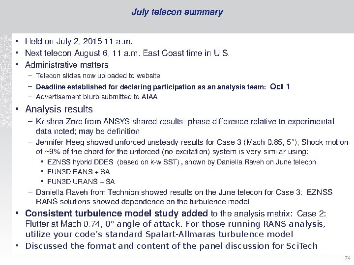
July telecon summary • Held on July 2, 2015 11 a. m. • Next telecon August 6, 11 a. m. East Coast time in U. S. • Administrative matters – Telecon slides now uploaded to website – Deadline established for declaring participation as an analysis team: Oct 1 – Advertisement blurb submitted to AIAA • Analysis results – Krishna Zore from ANSYS shared results- phase difference relative to experimental data noted; may be definition – Jennifer Heeg showed unforced unsteady results for Case 3 (Mach 0. 85, 5°); Shock motion of ~9% of the chord for the unforced (no excitation) system is very similar using: • EZNSS hybrid DDES (based on k-w SST) , shown by Daniella Raveh on June telecon • FUN 3 D RANS + SA • FUN 3 D URANS + SA – Daniella Raveh from Technion showed results on the June telecon for Case 3: EZNSS RANS solutions showed dependence on the turbulence model • Consistent turbulence model study added to the analysis matrix: Case 2: Flutter at Mach 0. 74, 0° angle of attack. For those running RANS analysis, utilize your code’s standard Spalart-Allmaras turbulence model • Discussed the format and content of the panel discussion for Sci. Tech 74

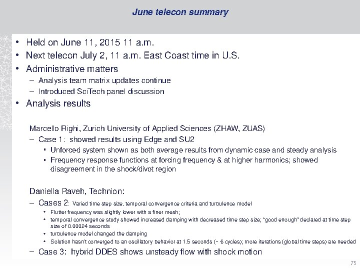
June telecon summary • Held on June 11, 2015 11 a. m. • Next telecon July 2, 11 a. m. East Coast time in U. S. • Administrative matters – Analysis team matrix updates continue – Introduced Sci. Tech panel discussion • Analysis results Marcello Righi, Zurich University of Applied Sciences (ZHAW, ZUAS) – Case 1: showed results using Edge and SU 2 • Unforced system shown as both average results from dynamic case and steady analysis • Frequency response functions at forcing frequency & at higher harmonics; showed disagreement in the shock/divot region Daniella Raveh, Technion: – Cases 2: Varied time step size, temporal convergence criteria and turbulence model • Flutter frequency was slightly lower with a finer mesh; • temporal convergence study showed increased damping with decreased time step size; “good enough” declared at time step size of 0. 00024 seconds • turbulence model changed the damping • Solution hasn’t converged to an oscillatory behavior at 1. 5 seconds (~ 6 cycles); more iterations (global time steps) are needed – Case 3: hybrid DDES shows unsteady flow with shock motion 75

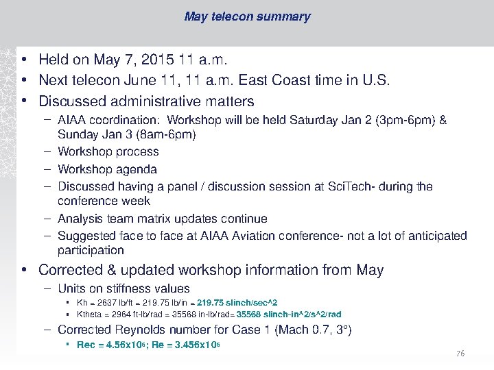
May telecon summary • Held on May 7, 2015 11 a. m. • Next telecon June 11, 11 a. m. East Coast time in U. S. • Discussed administrative matters – AIAA coordination: Workshop will be held Saturday Jan 2 (3 pm-6 pm) & Sunday Jan 3 (8 am-6 pm) – Workshop process – Workshop agenda – Discussed having a panel / discussion session at Sci. Tech- during the conference week – Analysis team matrix updates continue – Suggested face to face at AIAA Aviation conference- not a lot of anticipated participation • Corrected & updated workshop information from May – Units on stiffness values • Kh = 2637 lb/ft = 219. 75 lb/in = 219. 75 slinch/sec^2 • Ktheta = 2964 ft-lb/rad = 35568 in-lb/rad= 35568 slinch-in^2/s^2/rad – Corrected Reynolds number for Case 1 (Mach 0. 7, 3°) • Rec = 4. 56 x 106; Re = 3. 456 x 106 76

AIAA Interactions Approved and signed off by by Bruce Willis, Chairman of of Structural Dynamics Technical Committee Megan Scheidt, Managing Director of of Products and Programs 77

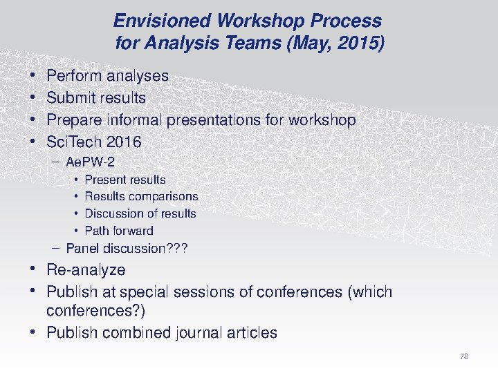
Envisioned Workshop Process for Analysis Teams (May, 2015) • • Perform analyses Submit results Prepare informal presentations for workshop Sci. Tech 2016 – Ae. PW-2 • • Present results Results comparisons Discussion of results Path forward – Panel discussion? ? ? • Re-analyze • Publish at special sessions of conferences (which conferences? ) • Publish combined journal articles 78

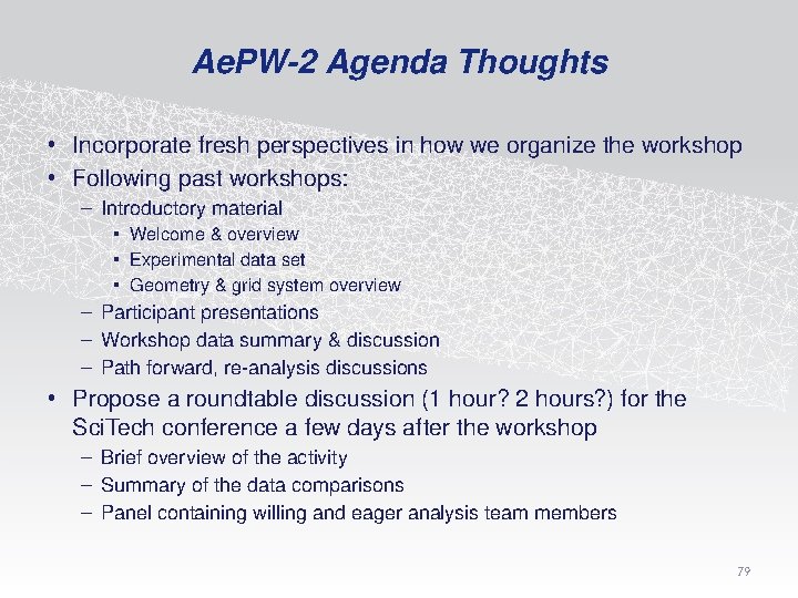
Ae. PW-2 Agenda Thoughts • Incorporate fresh perspectives in how we organize the workshop • Following past workshops: – Introductory material • Welcome & overview • Experimental data set • Geometry & grid system overview – Participant presentations – Workshop data summary & discussion – Path forward, re-analysis discussions • Propose a roundtable discussion (1 hour? 2 hours? ) for the Sci. Tech conference a few days after the workshop – Brief overview of the activity – Summary of the data comparisons – Panel containing willing and eager analysis team members 79

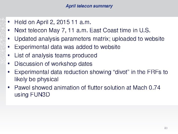
April telecon summary • • Held on April 2, 2015 11 a. m. Next telecon May 7, 11 a. m. East Coast time in U. S. Updated analysis parameters matrix; uploaded to website Experimental data was added to website List of analysis teams produced Discussion of workshop dates Experimental data reduction showing “divot” in the FRFs to likely be physical • Pawel showed animation of flutter solution at Mach 0. 74 using FUN 3 D 80

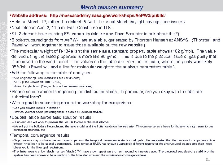
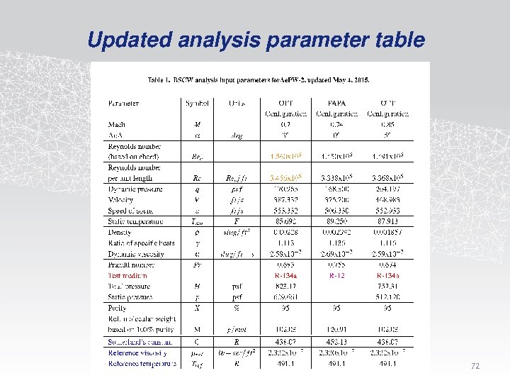
March telecon summary • Website address: http: //nescacademy. nasa. gov/workshops/Ae. PW 2/public/ • Held on March 12, rather than March 5 (with the usual March daylight savings time issues) • Next telecon April 2, 11 a. m. East Coast time in U. S. • SU-2 doesn’t have existing FSI capability. (Melike and Dave Schuster to talk about this? ) • Block-structured grids from Ae. PW-1 are available, generated by Thorsten Hansen at ANSYS. (Thorsten and Pawel will work together to make those available on the new website. ) • The molecular weight of R-134 a isn’t the same as a standard property table shows (102 g/mol). The value derived using the listed properties is more like 98 g/mol. This is due to the practical issue of gas purity that is achieved in the wind tunnel. The values on the table are from the test data, where the purity was likely 95%’ish. (Pawel will add a line for molecular weight to the analysis parameters table. ) • Add the following to the table of analyses: –ATA Engineering (Eric Blades will run Lo. Psi. Chem) –AFRL (Rick Graves will run FUN 3 D) –Milano Polytechnico (Sergio Ricci will run numerous codes) • Please send comments regarding the distributed slides. In particular, are you okay with the abstract submittal form? • With regard to submitting data to the workshop for comparison: –Can you provide results in matlab? –How do you feel about providing them in a data structure in matlab? • Doublet lattice aeroelastic solution results: –Bimo and Jen will work to present the results to date at the next telecon –We will put the bulk data file, including the aero model and the flutter cards on the web site. This can serve as a basis for those who might want to use correction methods, etc. • Temporal convergence results –Organizations may not have the resources to perform the temporal convergence study for all grids. It is suggested that this be done for a grid resolution where things look to be spatially converged. Experience at NASA has shown qualitatively different results for the unstructured coarse grid than those observed for the finer grid resolutions. –The flutter results at low Mach number (Mach 0. 74) have shown great variation with regard to time step size. The predicted aeroelasticity stability of the system has been shown to be a function of the time step size and the subiteration convergence level. 81

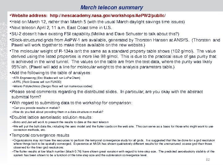
March telecon summary • Website address: http: //nescacademy. nasa. gov/workshops/Ae. PW 2/public/ • Held on March 12, rather than March 5 (with the usual March daylight savings time issues) • Next telecon April 2, 11 a. m. East Coast time in U. S. • SU-2 doesn’t have existing FSI capability. (Melike and Dave Schuster to talk about this? ) • Block-structured grids from Ae. PW-1 are available, generated by Thorsten Hansen at ANSYS. (Thorsten and Pawel will work together to make those available on the new website. ) • The molecular weight of R-134 a isn’t the same as a standard property table shows (102 g/mol). The value derived using the listed properties is more like 98 g/mol. This is due to the practical issue of gas purity that is achieved in the wind tunnel. The values on the table are from the test data, where the purity was likely 95%’ish. (Pawel will add a line for molecular weight to the analysis parameters table. ) • Add the following to the table of analyses: –ATA Engineering (Eric Blades will run Lo. Psi. Chem) –AFRL (Rick Graves will run FUN 3 D) –Milano Polytechnico (Sergio Ricci will run numerous codes) • Please send comments regarding the distributed slides. In particular, are you okay with the abstract submittal form? • With regard to submitting data to the workshop for comparison: –Can you provide results in matlab? –How do you feel about providing them in a data structure in matlab? • Doublet lattice aeroelastic solution results: –Bimo and Jen will work to present the results to date at the next telecon –We will put the bulk data file, including the aero model and the flutter cards on the web site. This can serve as a basis for those who might want to use correction methods, etc. • Temporal convergence results –Organizations may not have the resources to perform the temporal convergence study for all grids. It is suggested that this be done for a grid resolution where things look to be spatially converged. Experience at NASA has shown qualitatively different results for the unstructured coarse grid than those observed for the finer grid resolutions. –The flutter results at low Mach number (Mach 0. 74) have shown great variation with regard to time step size. The predicted aeroelasticity stability of the system has been shown to be a function of the time step size and the subiteration convergence level. 82

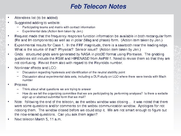
Feb Telecon Notes • • Attendees list (to be added) Suggested adding to website: – – • • Request made that the frequency response function information be available in both rectangular form (Re and Im components) as well as in polar (Mag and phase) form. (Action item taken by Jen. ) Experimental results for Case 1. In the FRF magnitude, there is a sawtooth near the leading edge. What is the source of that? Physical? Sensor issue? (Action item taken by Jen. ) Grids: structured grids were generated by NASA in plot 3 D format using Pointwise. The gridding guidelines still include the RSW and HIRENASD from Ae. PW-1. Need to revise them so that they are not confusing. Revisit them also with regard to the Reynolds number. Nonlinear effects and LCO: – – • • Discussion regarding hysteresis and identification of the neutral stability point Discussion about experimental data sets, including a DLR study on LCO where there were trends with Mach number Process: – – • Participating teams and matrix with contact information Experimental data (Action item taken by Jen. ) Think about what questions we are trying to answer How do we tell the organizing committee that we are participating by performing analyses? Is there a website sign up or abstract submittal form that we mail? Note: following the end of the telecon, as the webex window was closing… it was noted that there were some questions and/or comments on the webex communication window. Apologies for noticing them. The window closed before we could stop it. We are not smart enough to figure out the now-erased questions. Can you ask them again? Next telecon March 5, 11 a. m.

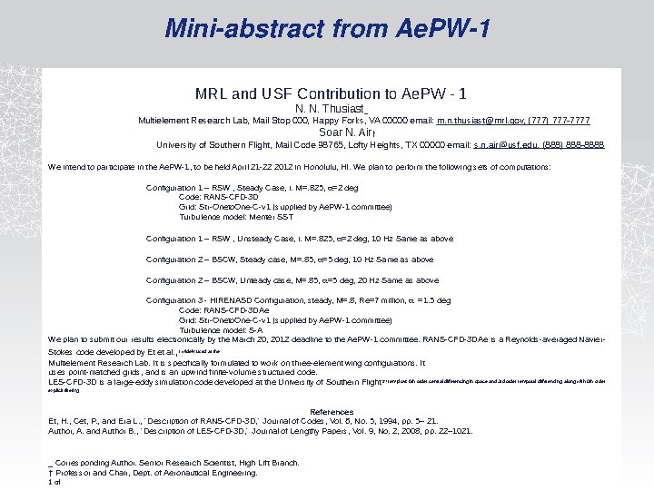
Mini-abstract from Ae. PW-1 MRL and USF Contribution to Ae. PW - 1 N. N. Thusiast_ Multielement Research Lab, Mail Stop 000, Happy Forks, VA 00000 email: m. n. thusiast@mrl. gov, (777) 777 -7777 Soar N. Air† University of Southern Flight, Mail Code 98765, Lofty Heights, TX 00000 email: s. n. air@usf. edu, (888) 888 -8888 We intend to participate in the Ae. PW-1, to be held April 21 -22 2012 in Honolulu, HI. We plan to perform the following sets of computations: Configuration 1 – RSW , Steady Case, i. M=. 825, =2 deg Code: RANS-CFD-3 D Grid: Str-Oneto. One-C-v 1 (supplied by Ae. PW-1 committee) Turbulence model: Menter SST Configuration 1 – RSW , Unsteady Case, i. M=. 825, =2 deg, 10 Hz Same as above Configuration 2 – BSCW, Steady case, M=. 85, =5 deg, 10 Hz Same as above Configuration 2 – BSCW, Unteady case, M=. 85, =5 deg, 20 Hz Same as above Configuration 3 - HIRENASD Configuration, steady, M=. 8, Re=7 million, =1. 5 deg Code: RANS-CFD-3 DAe Grid: Str-Oneto. One-C-v 1 (supplied by Ae. PW-1 committee) Turbulence model: S-A We plan to submit our results electronically by the March 20, 2012 deadline to the Ae. PW-1 committee. RANS-CFD-3 DAe is a Reynolds-averaged Navier. Stokes code developed by Et et al. , 1 widely used at the Multielement Research Lab. It is specifically formulated to work on three-element wing configurations. It uses point-matched grids, and is an upwind finite-volume structured code. LES-CFD-3 D is a large-eddy simulation code developed at the University of Southern Flight. 2 It employs 6 th order central differencing in space and 3 rd order temporal differencing, along with 9 th order explicit filtering. References Et, H. , Cet, P. , and Era L. , “Description of RANS-CFD-3 D, ” Journal of Codes, Vol. 6, No. 5, 1994, pp. 5– 21. Author, A. and Author B. , “Description of LES-CFD-3 D, ” Journal of Lengthy Papers, Vol. 9, No. 2, 2008, pp. 22– 1021. _ Corresponding Author. Senior Research Scientist, High Lift Branch. † Professor and Chair, Dept. of Aeronautical Engineering. 1 of 84