Working with astrometric data warnings and caveats X

Working with astrometric data - warnings and caveats X. Luri (U. Bastian) ESAC – November 2016

Scientist’s dream er av a ila ble • Error-free data • No random errors • No biases • No correlations Ne • Direct measurements • No transformations • No assumptions ve r ev • Complete sample • No censorships ESAC – November 2016

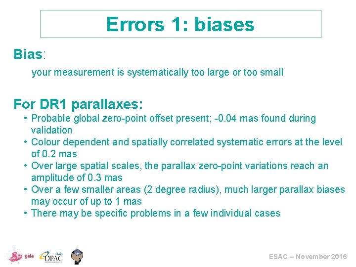
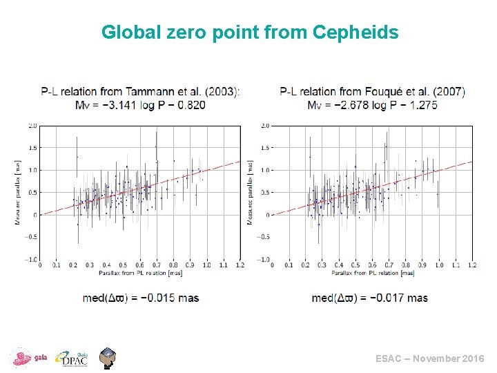
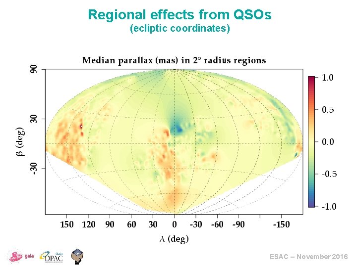
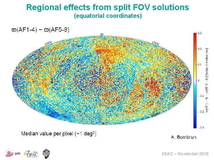
Errors 1: biases Bias: your measurement is systematically too large or too small For DR 1 parallaxes: • Probable global zero-point offset present; -0. 04 mas found during validation • Colour dependent and spatially correlated systematic errors at the level of 0. 2 mas • Over large spatial scales, the parallax zero-point variations reach an amplitude of 0. 3 mas • Over a few smaller areas (2 degree radius), much larger parallax biases may occur of up to 1 mas • There may be specific problems in a few individual cases ESAC – November 2016

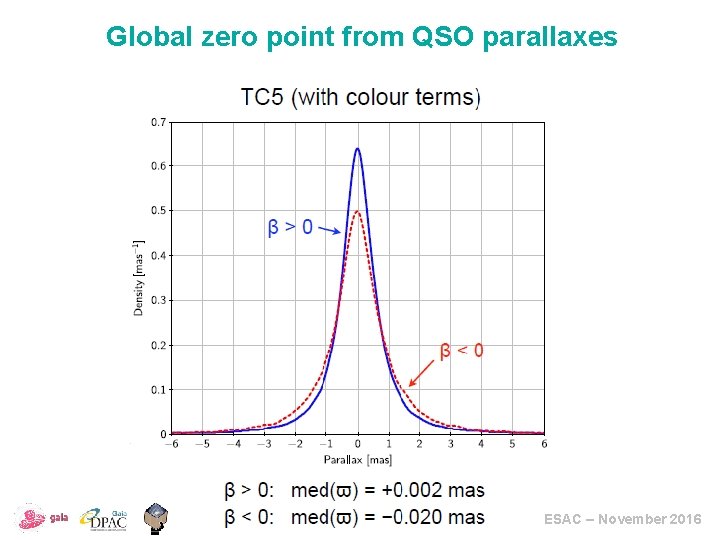
Global zero point from QSO parallaxes ESAC – November 2016

Global zero point from Cepheids ESAC – November 2016

Regional effects from QSOs (ecliptic coordinates) ESAC – November 2016

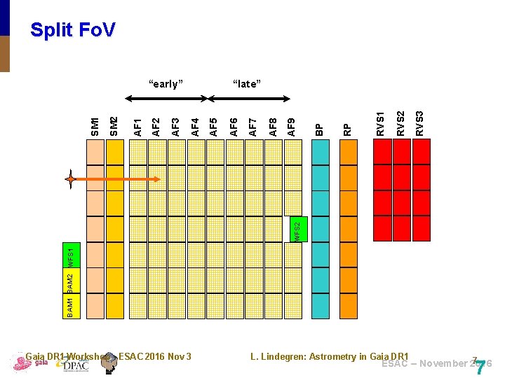
Split Fo. V RVS 3 RVS 2 RVS 1 RP BP AF 9 BAM 1 BAM 2 WFS 1 WFS 2 AF 8 AF 7 AF 6 AF 5 “late” AF 4 AF 3 AF 2 AF 1 SM 2 SM 1 “early” Gaia DR 1 Workshop - ESAC 2016 Nov 3 L. Lindegren: Astrometry in Gaia DR 1 7 ESAC – November 2016 7

Regional effects from split FOV solutions (equatorial coordinates) ESAC – November 2016

How to take this into account • You can introduce a global zero-point offset to use the parallaxes (suggested -0. 04 mas) • You cannot correct the regional features: if we could, we would already have corrected them. We have indications that these zero points may be present, but no more. • For most of the sky assume an additional systematic error of 0. 3 mas; your derived standard errors for anything cannot go below this value ϖ ± σϖ (random) ± 0. 3 mas (syst. ) • For a few smaller regions be aware that the systematics might reach 1 mas This is possibly the sole aspect in which Gaia DR 1 is not better than Hipparcos (apart from the incompleteness for the brightest stars) ESAC – November 2016

More specifically: treat separately random error and bias, but if you must combine them, a worst case formula can be as follows • For individual parallaxes: to be on the safe side add 0. 3 mas to the standard uncertainty Total sqrt( 2 Std+0. 32) • When averaging parallaxes for groups of stars: the random error will decrease as sqrt(N) but the systematic error (0. 3 mas) will not decrease final sqrt( 2 average. Std+0. 32) where average. Std decrease is the formal standard deviation of the average, computed in the usual way from the sigmas of the individual values in the average (giving essentially the sqrt(N) reduction). • Don’t try to get a “zonal correction” from previous figures, it’s too risky ESAC – November 2016

For DR 1 proper motions and positions: • In this case Gaia data is the best available, by far. • We do not have means to do a check as precise as the one done for parallaxes, but there are no indications of any significant bias • For positions remember that for comparison purposes you will likely have to convert them to another epoch. You should propagate the errors accordingly. ESAC – November 2016

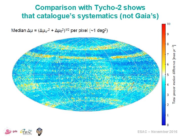
Comparison with Tycho-2 shows that catalogue’s systematics (not Gaia’s) ESAC – November 2016

Errors 2: random errors Random error: your measurements are randomly distributed around the true value • Each measurement in the catalogue comes with a formal error • Random errors in Gaia are quasi-normal. The formal error can be assimilated to the variance of a normal distribution around the true value. • Published formal errors for Gaia DR 1 may be slightly overestimated ESAC – November 2016

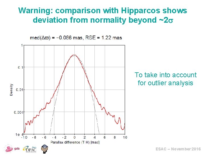
Warning: comparison with Hipparcos shows deviation from normality beyond ~2 To take into account for outlier analysis ESAC – November 2016

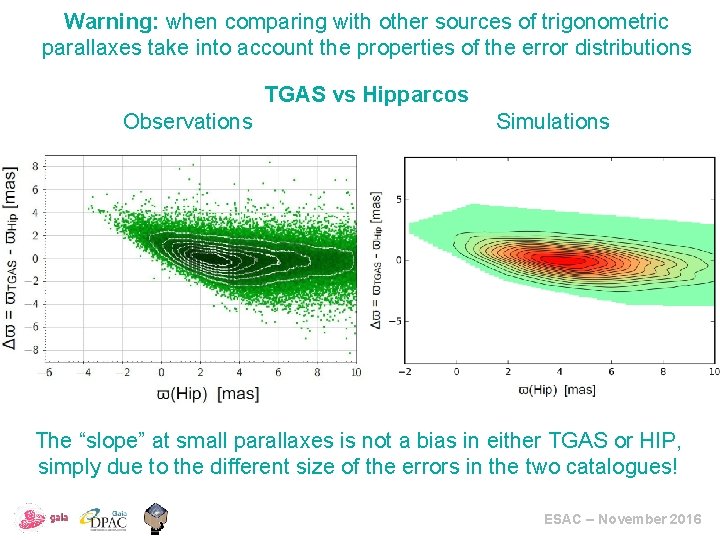
Warning: when comparing with other sources of trigonometric parallaxes take into account the properties of the error distributions TGAS vs Hipparcos Observations Simulations The “slope” at small parallaxes is not a bias in either TGAS or HIP, simply due to the different size of the errors in the two catalogues! ESAC – November 2016

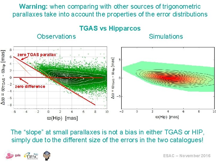
Warning: when comparing with other sources of trigonometric parallaxes take into account the properties of the error distributions TGAS vs Hipparcos Observations Simulations zero TGAS parallax zero difference The “slope” at small parallaxes is not a bias in either TGAS or HIP, simply due to the different size of the errors in the two catalogues! ESAC – November 2016

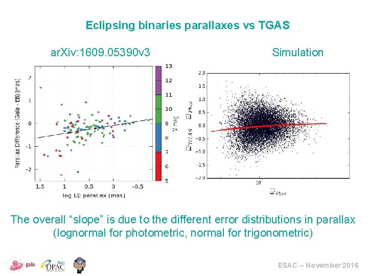
Eclipsing binaries parallaxes vs TGAS ar. Xiv: 1609. 05390 v 3 Simulation The overall “slope” is due to the different error distributions in parallax (lognormal for photometric, normal for trigonometric) ESAC – November 2016

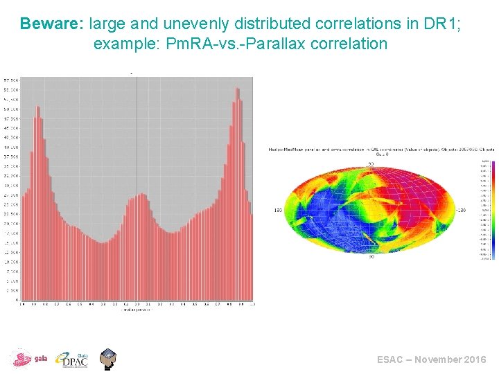
Errors 3: correlations Correlation: the measurements of several quantities are not independent from each other • Whenever you take linear combinations of such quantities, the correlations have to be taken into account in the error calculus ( and even more so for non-linear functions ) • The errors in the five astrometric parameters provided are not independent • The ten correlations between these parameters are provided in the Gaia DR 1 archives (correlation matrix) ESAC – November 2016

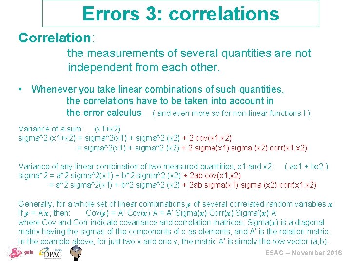
Errors 3: correlations Correlation: the measurements of several quantities are not independent from each other. • Whenever you take linear combinations of such quantities, the correlations have to be taken into account in the error calculus ( and even more so for non-linear functions ! ) Variance of a sum: (x 1+x 2) sigma^2 (x 1+x 2) = sigma^2(x 1) + sigma^2 (x 2) + 2 cov(x 1, x 2) = sigma^2(x 1) + sigma^2 (x 2) + 2 sigma(x 1) sigma (x 2) corr(x 1, x 2) Variance of any linear combination of two measured quantities, x 1 and x 2 : ( ax 1 + bx 2 ) sigma^2 = a^2 sigma^2(x 1) + b^2 sigma^2 (x 2) + 2 ab cov(x 1, x 2) = a^2 sigma^2(x 1) + b^2 sigma^2 (x 2) + 2 ab sigma(x 1) sigma (x 2) corr(x 1, x 2) Generally, for a whole set of linear combinations y of several correlated random variables x : If y = A’x, then: Cov(y) = A’ Cov(x) A = A’ Sigma(x) Corr(x) Sigma’(x) A where Cov and Corr indicate covariance and correlation matrices, Sigma(x) is a diagonal matrix having the sigmas of the components of x as elements, and A’ is the relation matrix. In the example above, for just two x and one y, the matrix A’ is simply the row vector (a, b). ESAC – November 2016

Examples of problematic use: • Simple epoch propagation (!) pos&pm • Calculation of proper directions pos&pm&parallax • Proper motion in a given direction on the sky (other than north-south or east-west) proper-motion components • Proper motion components in galactic or ecliptic coordinates proper-motion components • More complex, non-linear example: Calculating the transversal velocities of a set of stars • The resulting dispersion of velocities is influenced by the errors in parallax and in proper motion; thus 3 -dimensional case. • Its determination can not be done using the parallax and proper motion errors separately; the correlations have to be taken into account • But this time it’s non-linear! The error distribution will no longer be Gaussian. • The A matrix of the previous page will become the Jacobian matrix of the local derivatives of the transversal velocity wrt parallax and pm components ESAC – November 2016

Beware: large and unevenly distributed correlations in DR 1; example: Pm. RA-vs. -Parallax correlation ESAC – November 2016

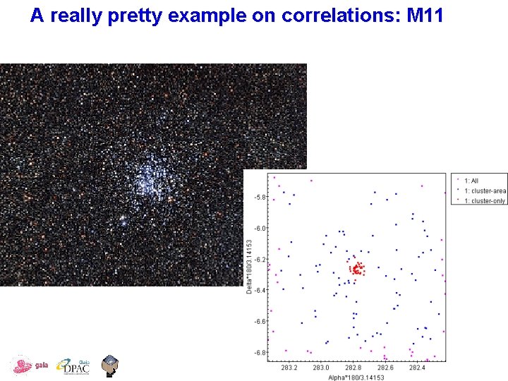
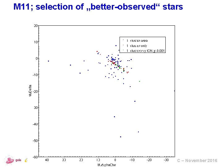
A really pretty example on correlations: M 11 ESAC – November 2016

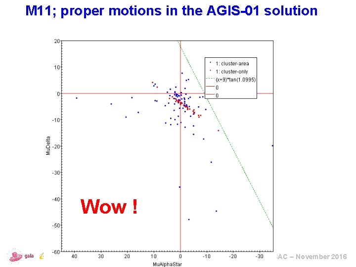
M 11; proper motions in the AGIS-01 solution Wow ! ESAC – November 2016

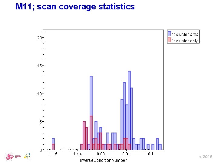
M 11; scan coverage statistics ESAC – November 2016

M 11; selection of „better-observed“ stars Wow ! ESAC – November 2016

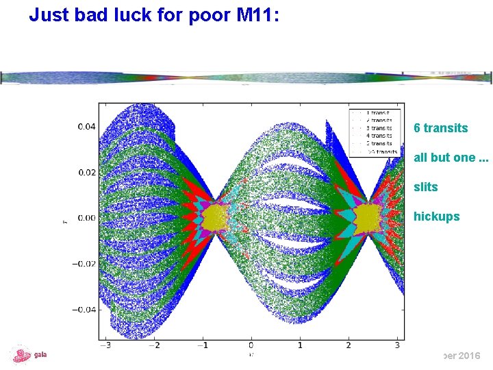
Just bad luck for poor M 11: 6 transits all but one. . . slits hickups ESAC – November 2016

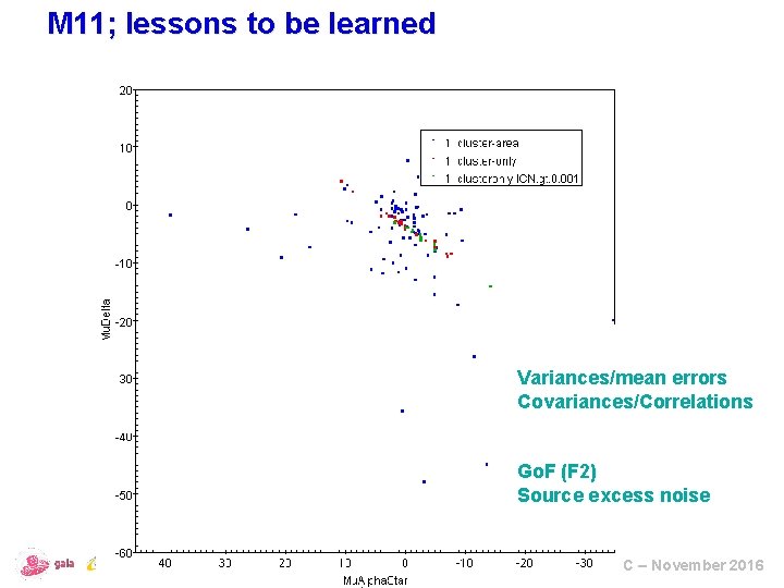
M 11; lessons to be learned Variances/mean errors Covariances/Correlations Wow ! Go. F (F 2) Source excess noise ESAC – November 2016

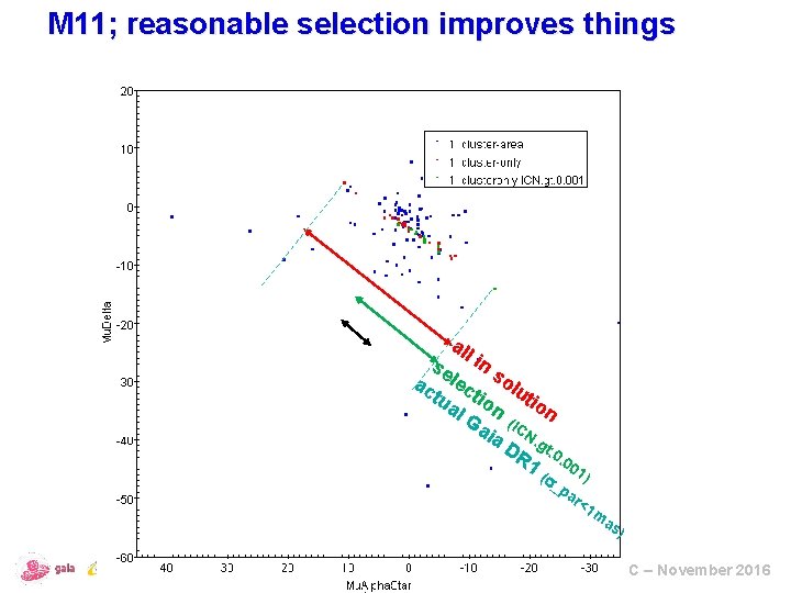
M 11; reasonable selection improves things all Wow ! se in s ac lec olu tu tio t al n ion Ga (IC ia N. g DR t. 0 1 (. 001 _ ) pa r< 1 m as ) ESAC – November 2016

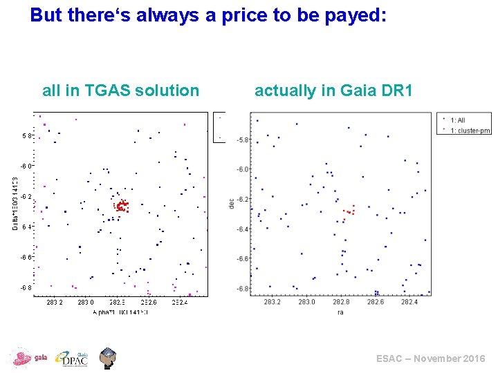
But there‘s always a price to be payed: all in TGAS solution actually in Gaia DR 1 ESAC – November 2016

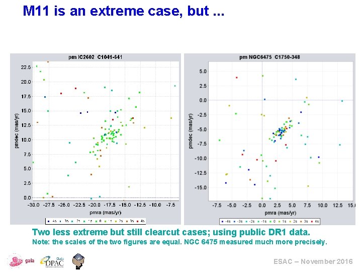
M 11 is an extreme case, but. . . Two less extreme but still clearcut cases; using public DR 1 data. Note: the scales of the two figures are equal. NGC 6475 measured much more precisely. ESAC – November 2016

Chapter 4: Transformations: when the quantity you want to study is not the quantity you observe • Usually you want distances, not parallaxes • Usually you want spatial velocities, not proper motions ESAC – November 2016

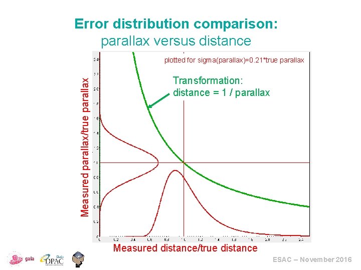
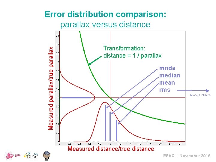
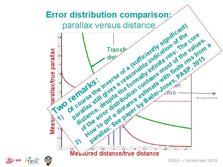
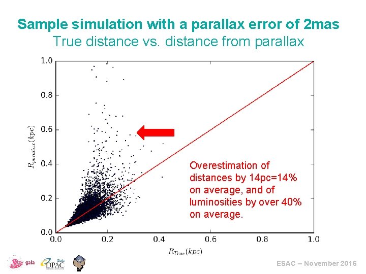
Warning: when using a transformed quantity the error distribution also is transformed • This is especially crucial for the calculation of distances from parallaxes • And even more so for the calculation of luminosities from parallaxes • A symmetrical, well behaved error in parallax is transformed into an asymmetrical error in distance ESAC – November 2016

Error distribution comparison: parallax versus distance Measured parallax/true parallax plotted for sigma(parallax)=0. 21*true parallax Transformation: distance = 1 / parallax Measured distance/true distance ESAC – November 2016

Measured parallax/true parallax Error distribution comparison: parallax versus distance Transformation: distance = 1 / parallax mode median mean rms always infinite Measured distance/true distance ESAC – November 2016

Error distribution comparison: parallax versus distance Measured parallax/true parallax t) n a c i if the ore. n ig of e c es s a n Th alu y l o t i Transformation: n at : e v rom s e i ic rm th s f distance = 1 ff/icparallax d n ite of rm 015 i u s le in st te 2 ( , f b i o a f na in mmode in SP f o y o h PA e as all ins median t i s r re m ta w s, : e e s inv s a for con ate omean n k ar the give the tion stim ler-J rms m rse ill pite bu e e ai always infinite e r ou st es tri nc y B o c lax , d dis sta r b f w T O aral nce rror a di ape p sta e et p 1) e i e d th o g Se of w t ax: Ho rall pa 2) Measured distance/true distance ESAC – November 2016

Sample simulation with a parallax error of 2 mas True distance vs. distance from parallax Overestimation of distances by 14 pc=14% on average, and of luminosities by over 40% on average. ESAC – November 2016

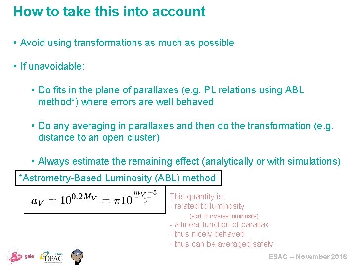
How to take this into account • Avoid using transformations as much as possible • If unavoidable: • Do fits in the plane of parallaxes (e. g. PL relations using ABL method*) where errors are well behaved • Do any averaging in parallaxes and then do the transformation (e. g. distance to an open cluster) • Always estimate the remaining effect (analytically or with simulations) *Astrometry-Based Luminosity (ABL) method This quantity is: - related to luminosity (sqrt of inverse luminosity) - a linear function of parallax - thus nicely behaved - thus can be averaged safely ESAC – November 2016

Also beware of additional assumptions • For instance about the absorption when calculating absolute magnitudes from parallaxes ESAC – November 2016

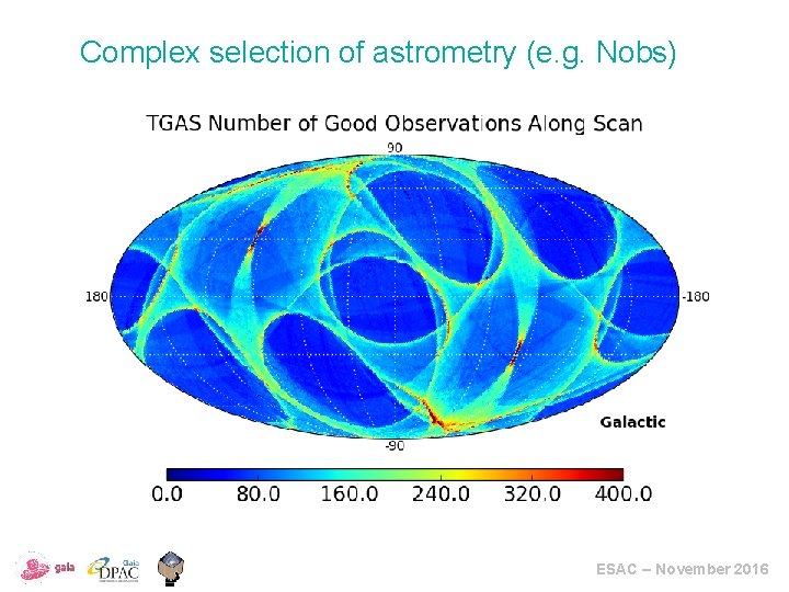
Chapter 5: Sample censorships Completeness/representativeness: we have the complete population of objects or at least a subsample which is representative for a given purpose • DR 1 is a very complex dataset, its completeness or representativeness can not be guaranteed for any specific purpose ESAC – November 2016

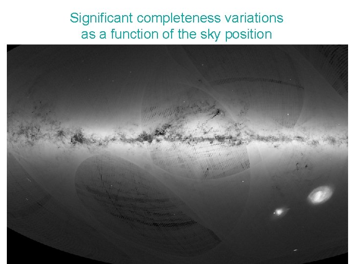
Significant completeness variations as a function of the sky position ESAC – November 2016

Complex selection of astrometry (e. g. Nobs) ESAC – November 2016

How to take this into account • Very difficult, will depend on your specific purpose • Analyze if the problem exists, and try to determine if the known censorships are correlated with the parameter you are analyzing (see validation paper) • At least do some simulations to evaluate the possible effects ESAC – November 2016

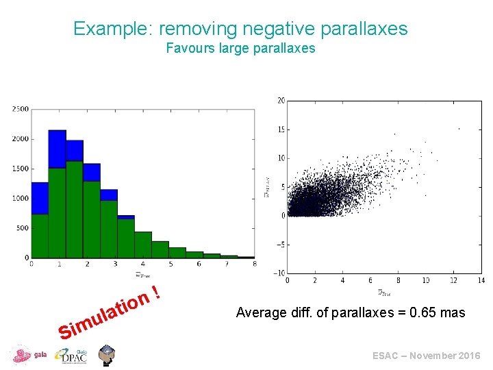
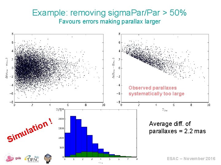
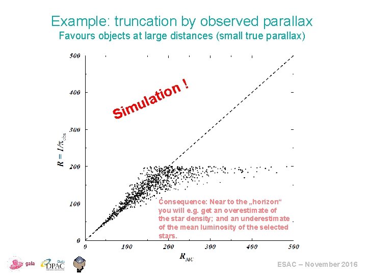
IMPORTANT: do not make things worse by adding your own additional censorships • This is specially important for parallaxes • Avoid removing negative parallaxes; this removes information and biases the sample for distant stars • Avoid selecting subsamples on parallax relative error. This also removes information and biases the sample for distant stars • Use instead fitting methods able to use all available data (e. g. Bayesian methods) and always work on the observable space (e. g. on parallaxes, not on distances or luminosities) ESAC – November 2016

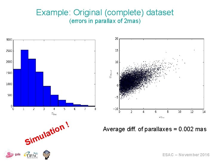
Example: Original (complete) dataset (errors in parallax of 2 mas) S l u im ! n atio Average diff. of parallaxes = 0. 002 mas ESAC – November 2016

Example: removing negative parallaxes Favours large parallaxes Sim ! n o i t a ul Average diff. of parallaxes = 0. 65 mas ESAC – November 2016

Example: removing sigma. Par/Par > 50% Favours errors making parallax larger Observed parallaxes systematically too large ! n tio la u im Average diff. of parallaxes = 2. 2 mas S ESAC – November 2016

Example: truncation by observed parallax Favours objects at large distances (small true parallax) ! n atio S l u im Consequence: Near to the „horizon“ you will e. g. get an overestimate of the star density; and an underestimate of the mean luminosity of the selected stars. ESAC – November 2016

Appendix ESAC – November 2016

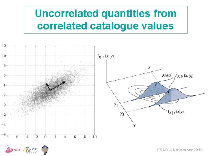
Uncorrelated quantities from correlated catalogue values ESAC – November 2016

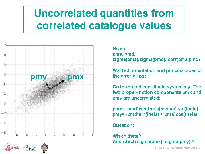
Uncorrelated quantities from correlated catalogue values Given: pma, pmd, sigma(pma), sigma(pmd), corr(pma, pmd) pmy pmx Wanted: orientation and principal axes of the error ellipse Go to rotated coordinate system x, y. The two proper-motion components pmx and pmy are uncorrelated: pmx= pmd*cos(theta) + pma* sin(theta) pmy= -pmd*sin(theta) + pma*cos(theta) Question: Which theta? And which sigma(pmx), sigma(pmy) ? ESAC – November 2016

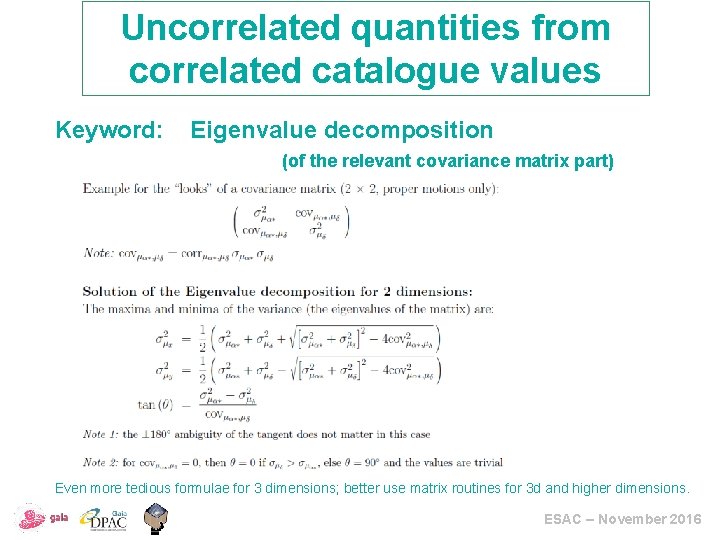
Uncorrelated quantities from correlated catalogue values Keyword: Eigenvalue decomposition (of the relevant covariance matrix part) Even more tedious formulae for 3 dimensions; better use matrix routines for 3 d and higher dimensions. ESAC – November 2016

Thank you ESAC – November 2016

During this presentation - about 1 million stars were measured by Gaia, - roughly 10 million astrometric measurements were taken, - about 300, 000 spectra were made of 100, 000 stars ESAC – November 2016