Working Scientifically Gradients on graphs Learning Objectives You

Working Scientifically: Gradients on graphs

Learning Objectives You should learn : • How to calculate the gradient (slope) of a straight-line graph… • …and a curved graph • About the equations for different straight-line graphs. • The meaning of gradients on graphs for distance‒time and velocity‒time.
Looking at graphs What do we mean by… …the gradient of a graph…?
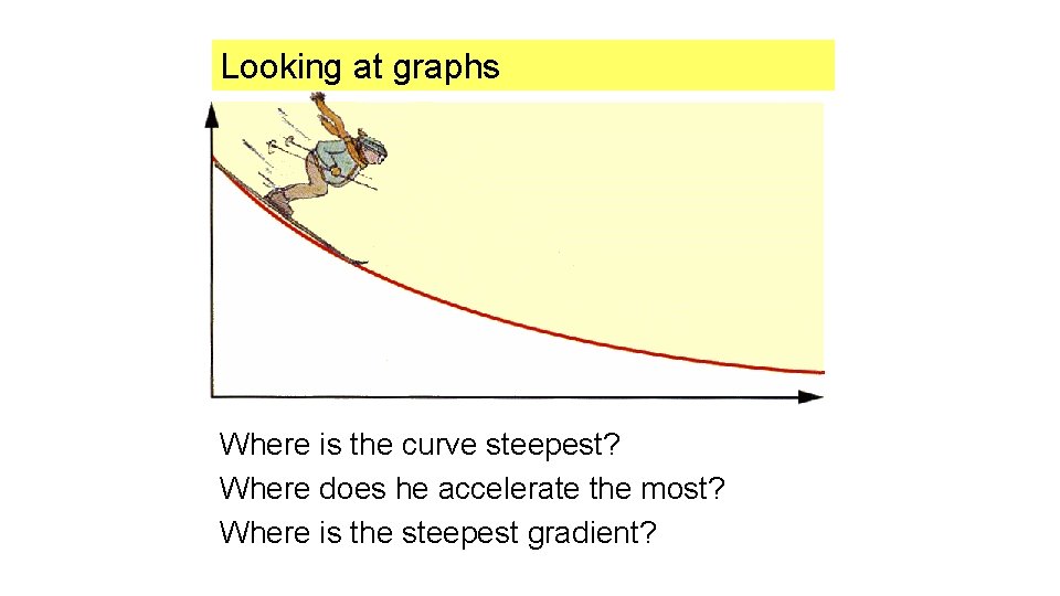
Looking at graphs Where is the curve steepest? Where does he accelerate the most? Where is the steepest gradient?
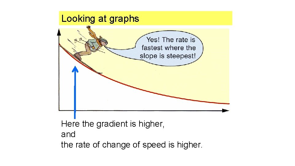
Looking at graphs Here the gradient is higher, and the rate of change of speed is higher.
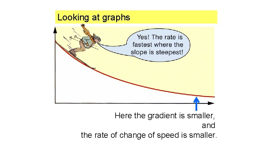
Looking at graphs Here the gradient is smaller, and the rate of change of speed is smaller.
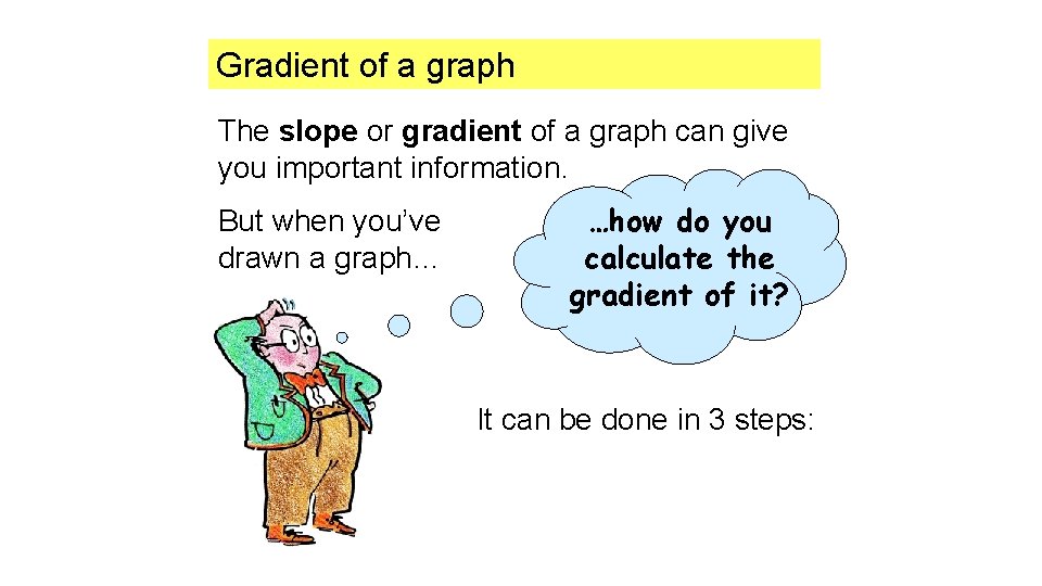
Gradient of a graph The slope or gradient of a graph can give you important information. But when you’ve drawn a graph… …how do you calculate the gradient of it? It can be done in 3 steps:
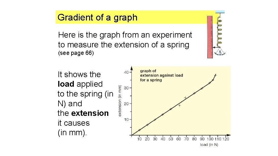
Gradient of a graph Here is the graph from an experiment to measure the extension of a spring (see page 66) It shows the load applied to the spring (in N) and the extension it causes (in mm).
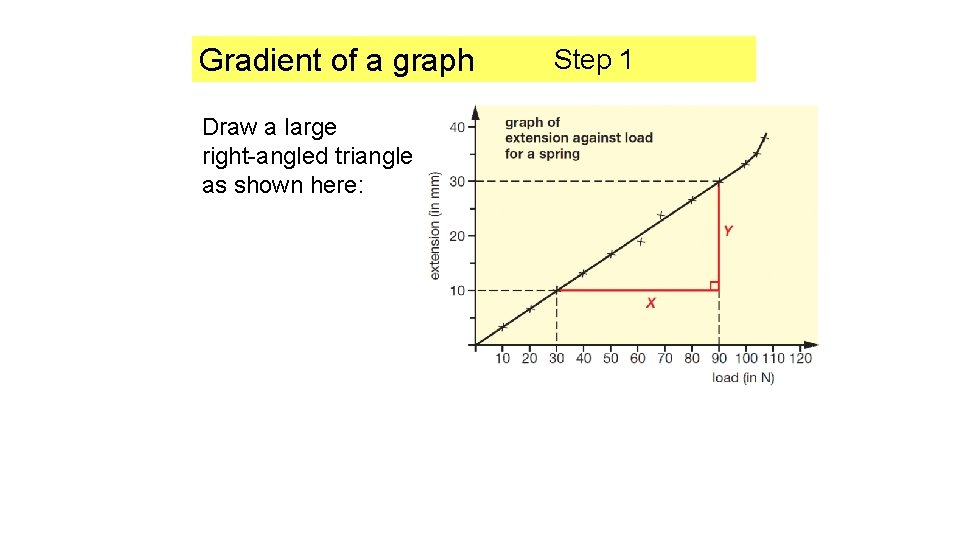
Gradient of a graph Draw a large right-angled triangle as shown here: Step 1
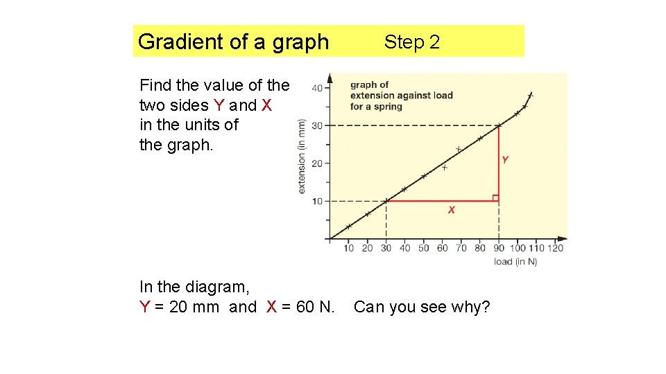
Gradient of a graph Step 2 Find the value of the two sides Y and X in the units of the graph. In the diagram, Y = 20 mm and X = 60 N. Can you see why?
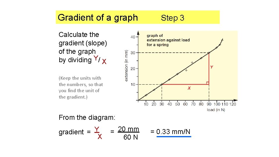
Gradient of a graph Step 3 Calculate the gradient (slope) of the graph by dividing Y/ X (Keep the units with the numbers, so that you find the unit of the gradient. ) From the diagram: gradient = Y X = 20 mm 60 N = 0. 33 mm/N
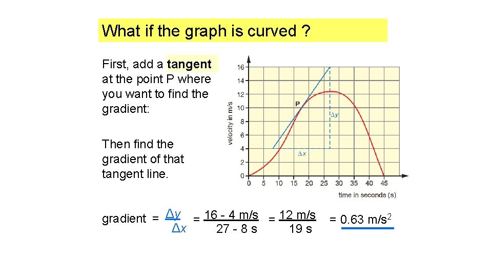
What if the graph is curved ? First, add a tangent at the point P where you want to find the gradient: Then find the gradient of that tangent line. gradient = Δy = 16 - 4 m/s = 12 m/s Δx 19 s 27 - 8 s = 0. 63 m/s 2
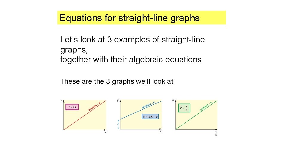
Equations for straight-line graphs Let’s look at 3 examples of straight-line graphs, together with their algebraic equations. These are the 3 graphs we’ll look at:
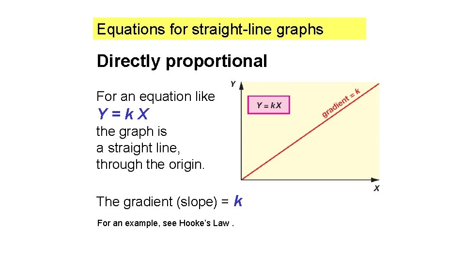
Equations for straight-line graphs Directly proportional For an equation like Y=k. X the graph is a straight line, through the origin. The gradient (slope) = k For an example, see Hooke’s Law.
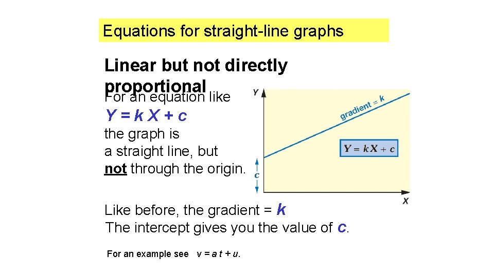
Equations for straight-line graphs Linear but not directly proportional For an equation like Y=k. X+c the graph is a straight line, but not through the origin. Like before, the gradient = k The intercept gives you the value of c. For an example see v = a t + u.
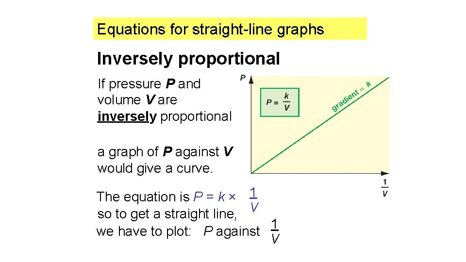
Equations for straight-line graphs Inversely proportional If pressure P and volume V are inversely proportional a graph of P against V would give a curve. The equation is P = k × 1 so to get a straight line, V 1 we have to plot: P against V
Looking at graphs of movement Let’s look at some examples of graphs with different gradients…

Distance – time graphs Example 1
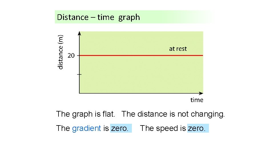
Distance – time graph The What graph is happening is flat. The here? distance is not changing. The gradient is zero. The speed is zero.

Distance – time graphs Example 2
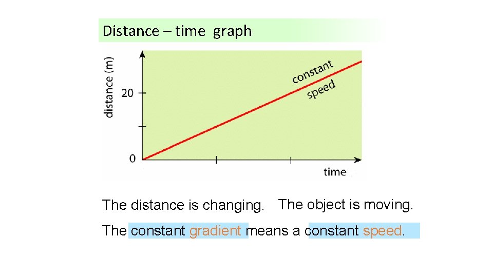
Distance – time graph What The distance is happening is changing. here? The object is moving. The constant gradient means a constant speed.
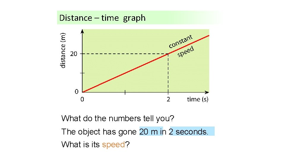
Distance – time graph What do the numbers tell you? The object has gone 20 m in 2 seconds. What is its speed?
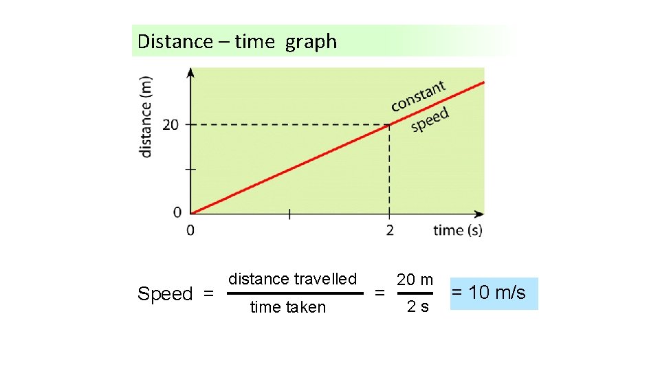
Distance – time graph Speed = distance travelled time taken = 20 m 2 s = 10 m/s
Distance – time graphs Example 3
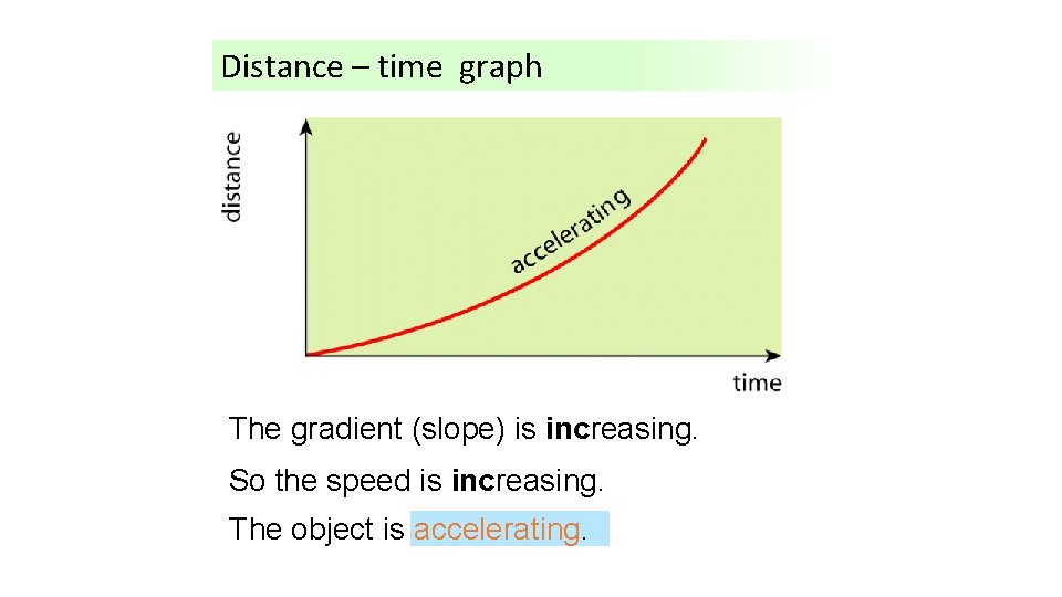
Distance – time graph The Whatgradient is happening (slope)here? is increasing. So the speed is increasing. The object is accelerating.

Distance – time graphs Example 4
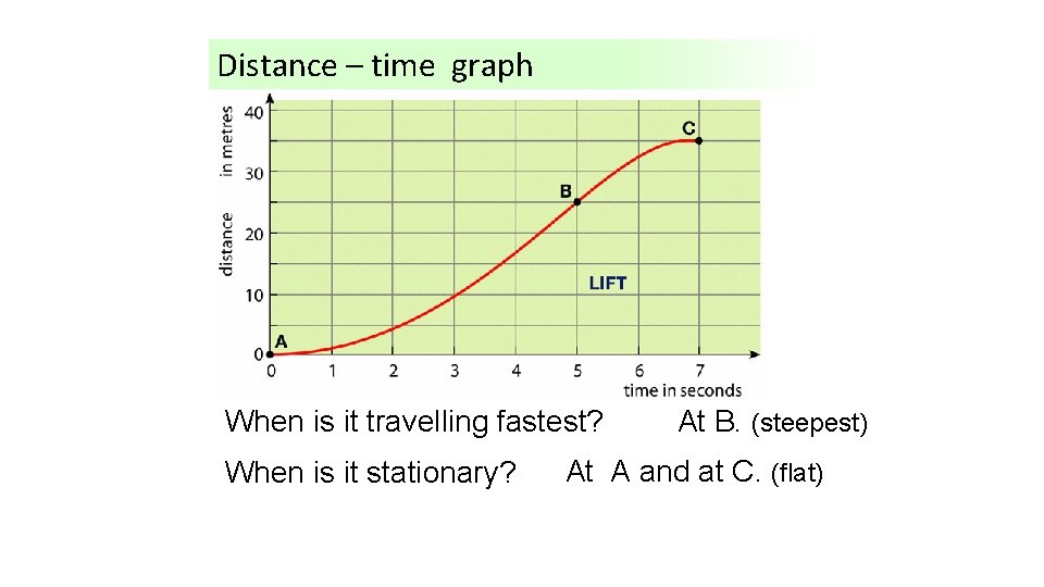
Distance – time graph When What isishappening it travellingtofastest? the lift? When is it stationary? At B. (steepest) At A and at C. (flat)
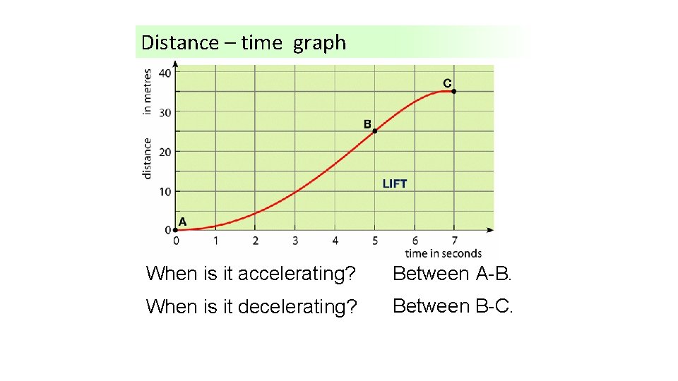
Distance – time graph When is it accelerating? Between A-B. When is it decelerating? Between B-C.
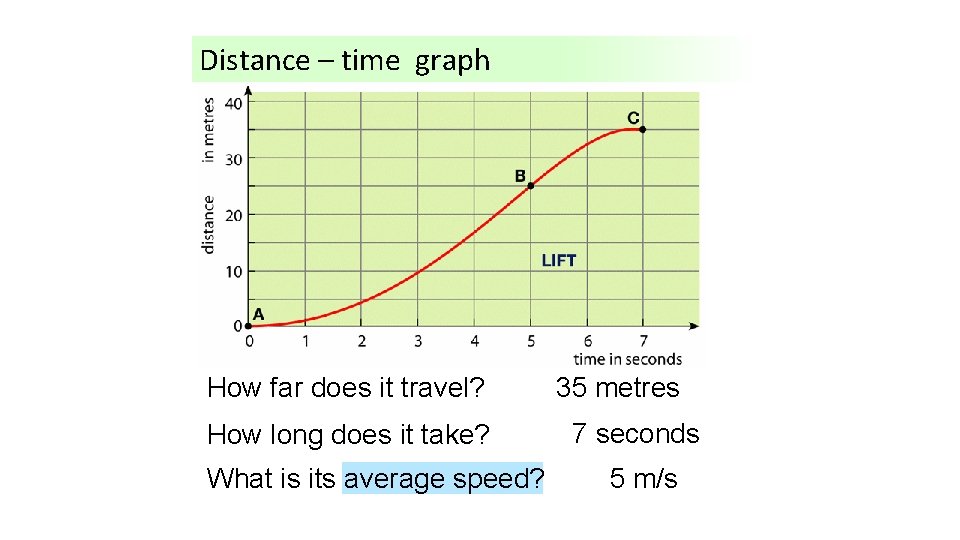
Distance – time graph How far does it travel? How long does it take? What is its average speed? 35 metres 7 seconds 5 m/s
Now let’s look at a different set of graphs… …graphs of velocity) against time

Velocity – time graph Example 1
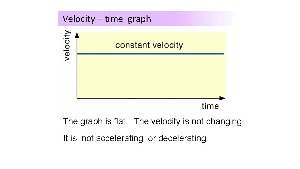
Velocity – time graph The Whatgraph is happening is flat. The here? velocity is not changing. It is not accelerating or decelerating.

Velocity – time graph Example 2
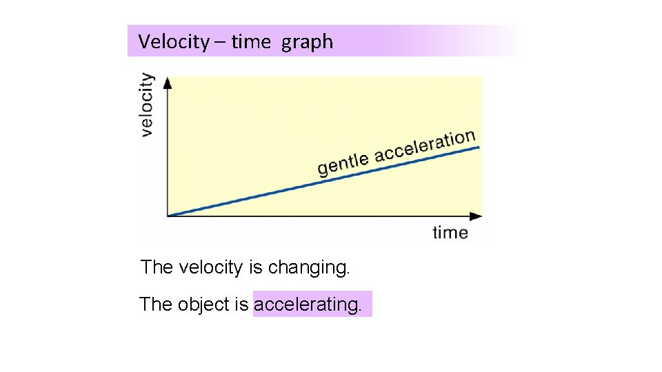
Velocity – time graph What The velocity is happening is changing. here? The object is accelerating.

Velocity – time graph Example 3
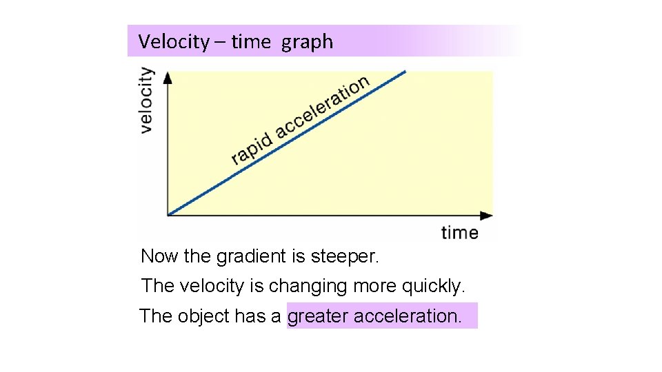
Velocity – time graph Now the gradient is steeper. The velocity is changing more quickly. The object has a greater acceleration.

Velocity – time graph Example 4
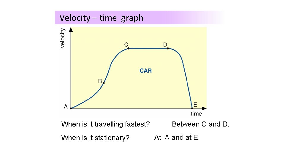
Velocity – time graph When travelling fastest? What isisithappening to this car? Between C and D. When is it stationary? At A and at E.
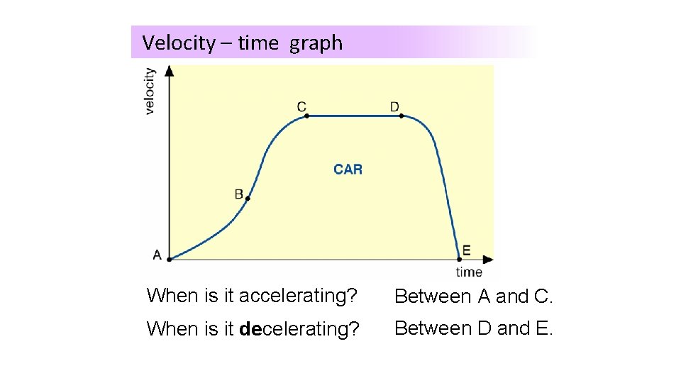
Velocity – time graph When is it accelerating? Between A and C. When is it decelerating? Between D and E.
Velocity – time graph Example 5
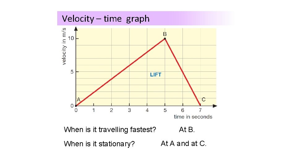
Velocity – time graph When travelling fastest? What isisithappening to this lift? At B. When is it stationary? At A and at C.
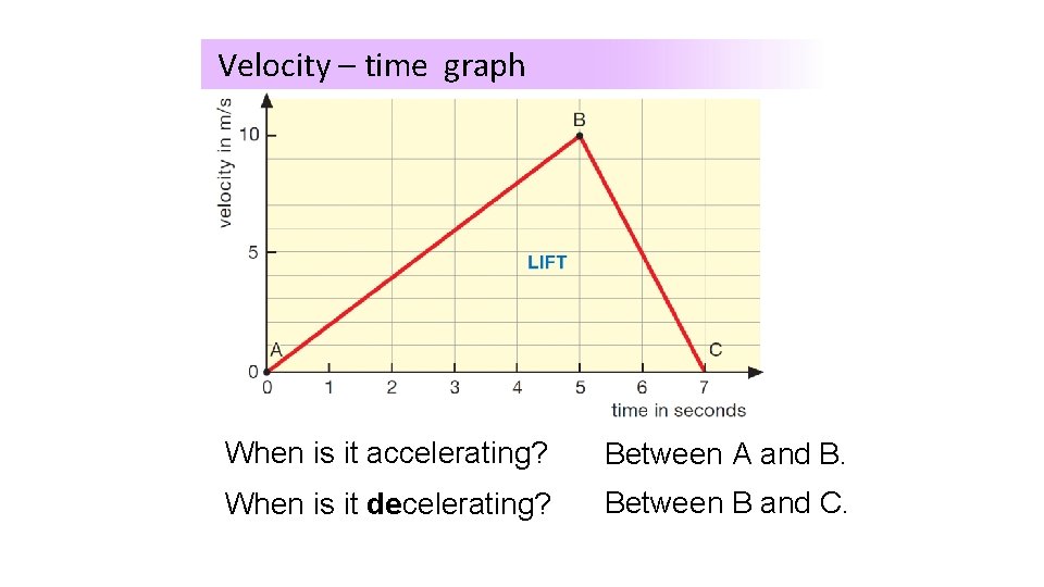
Velocity – time graph When is it accelerating? Between A and B. When is it decelerating? Between B and C.
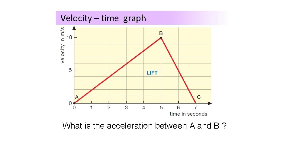
Velocity – time graph What is the acceleration between A and B ?
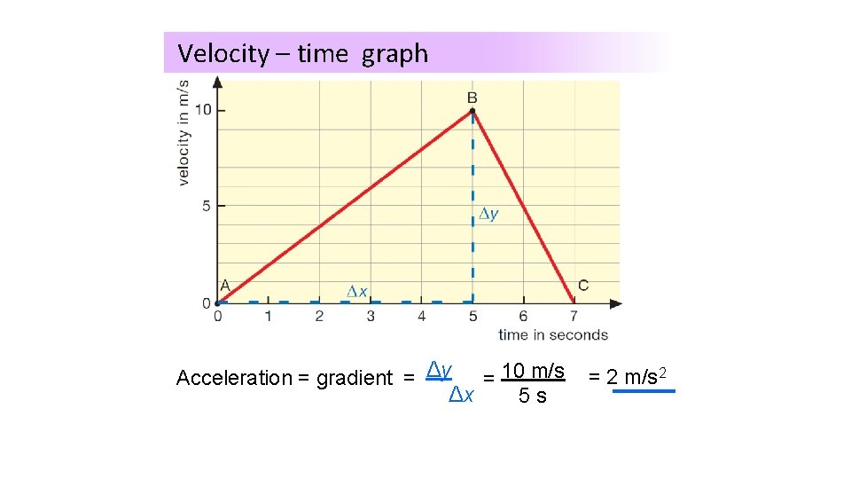
Velocity – time graph Acceleration = gradient = Δy = 10 m/s Δx 5 s = 2 m/s 2

Velocity – time graph What is the deceleration between B and C ?
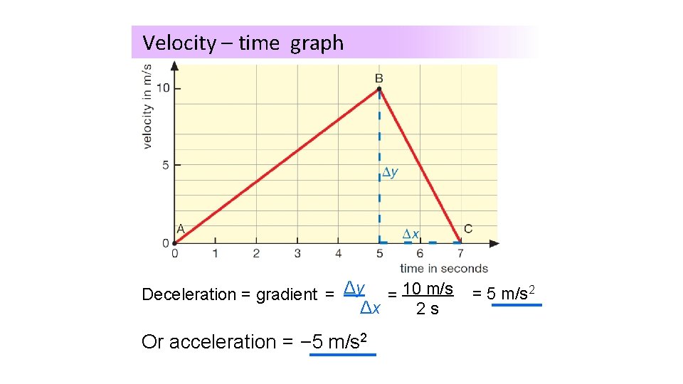
Velocity – time graph Deceleration = gradient = Δy = 10 m/s Δx 2 s Or acceleration = ‒ 5 m/s 2 = 5 m/s 2
Drawing a conclusion Every experiment has a ‘conclusion'. This is a summary of what you found out(or sometimes what you didn’t find). Always look at your results or graph or chart to decide what you have discovered. What reliable and valid deduction can be made from your results? What pattern can you see? If possible, try to use your scientific knowledge to explain and justify your conclusion.
Evaluating your evidence As part of the conclusion, comment should be made on the reliability and validity of the measurements that are made. The following can improve the reliability of the data: § Taking more measurements, perhaps changing the range. § Improving the design of the investigation. § Checking the results by an alternative method. § Looking up data from secondary sources(eg. Books or internet) § Seeing if other people following your method get the same results(i. e are your results reproducible)
- Slides: 48