Word Spotting DTW Word Spot DTW Introduction The

Word Spotting DTW

Word Spot DTW �Introduction �The Basic Idea �Pruning �DTW �Matching Words With DTW �Experimental Results �Summary

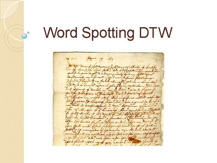
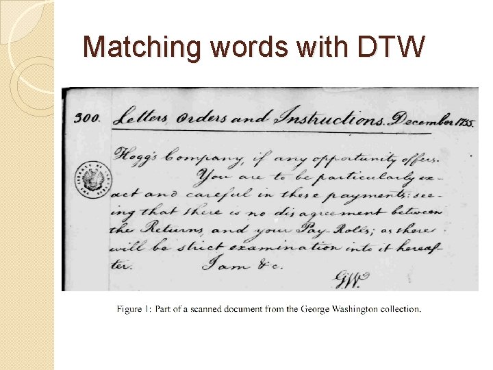
Introduction �Libraries contain an enormous amount of hand-written historical documents. �They would like to make it available electronically. �such large collections can only be accessed efficiently if a searchable index exist. �The current state-of-the-art approach is to manually create an index.

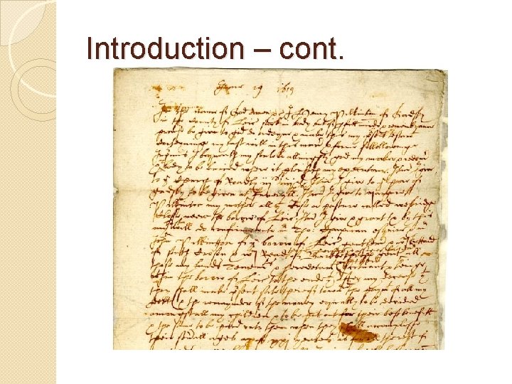
Introduction – cont. �The quality of historical documents is degraded due to faded ink, stained paper, etc. �Traditional Optical Character Recognition (OCR) techniques that usually recognize words character-bycharacter, fail.

Introduction – cont.

The Basic Idea �For handwritten manuscripts written by a single author - the images of multiple instances of the same word are likely to look similar. �Word spotting idea provides an alternative approach to index generation.

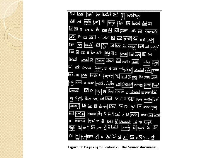
Word Spotting �Each page in the document collection is segmented into words. �The different instances of a word are clustered together using image matching. �A human can tag the n most interesting clusters for indexing with the appropriate ASCII equivalent.

Matching �Good matching performance can be achieved by: ◦ A technique that skews, resizes and aligns two candidate words. ◦ Compares the words pixel-by-pixel. �We will use DTW.

Pruning �Running a matching algorithm is expensive with growing collection sizes. �Pruning techniques which can discard unlikely matches are used.

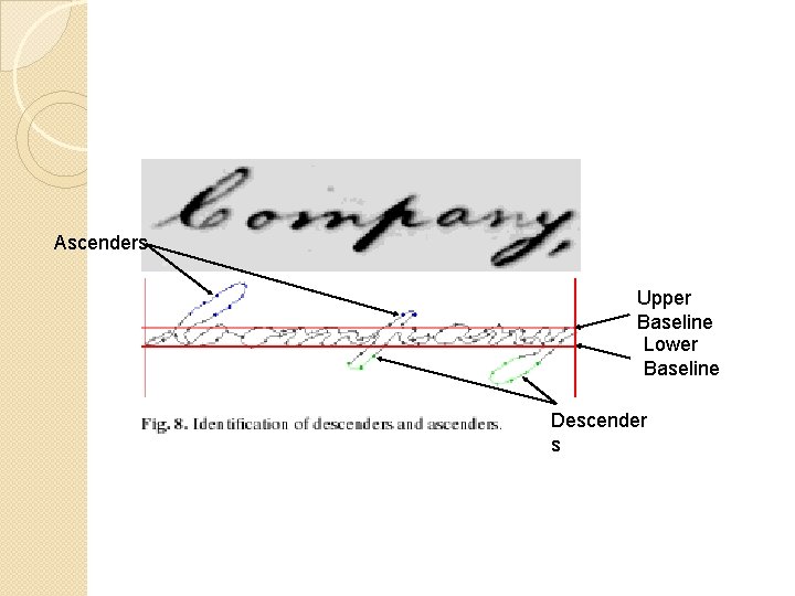
Pruning Techniques �Pruning of word pairs based on the area and aspect ratio of their bounding boxes. �Require words to have the same number of descenders (strokes below the baseline). �The idea is to require similar pruning statistics.

Ascenders Upper Baseline Lower Baseline Descender s

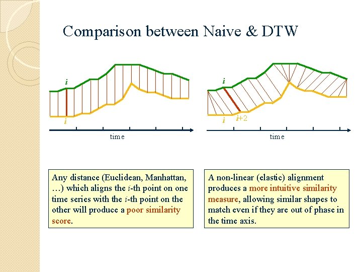
DTW �Used to compute a distance between two time series. �A time series is a list of samples taken from a signal ordered by time. �Naive approach: resample one of them and then compare the series sample-bysample. �does not produce intuitive results, as it compares samples that might not correspond well.

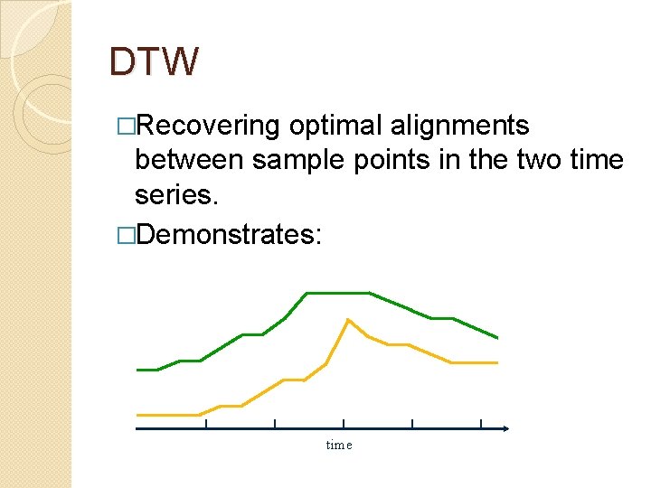
DTW �Recovering optimal alignments between sample points in the two time series. �Demonstrates: time

Comparison between Naive & DTW i i time Any distance (Euclidean, Manhattan, …) which aligns the i-th point on one time series with the i-th point on the other will produce a poor similarity score. i+2 time A non-linear (elastic) alignment produces a more intuitive similarity measure, allowing similar shapes to match even if they are out of phase in the time axis.

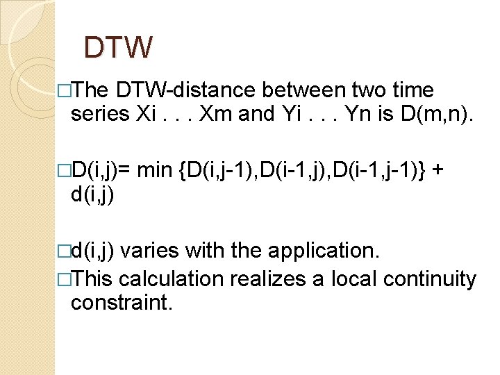
DTW �The DTW-distance between two time series Xi. . . Xm and Yi. . . Yn is D(m, n). �D(i, j)= d(i, j) �d(i, j) min {D(i, j-1), D(i-1, j-1)} + varies with the application. �This calculation realizes a local continuity constraint.

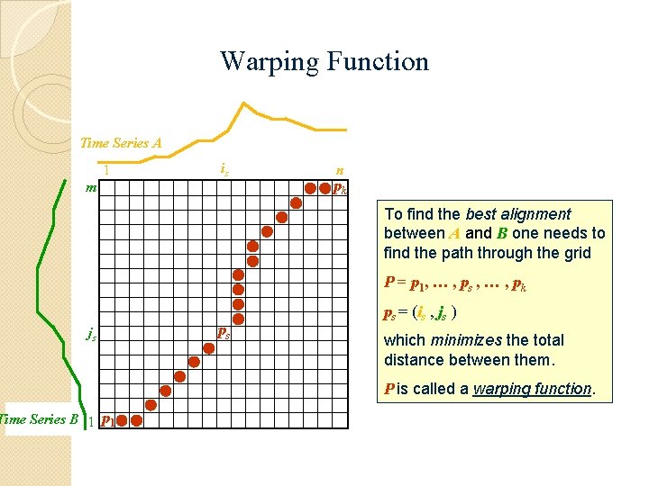
Warping Function Time Series A 1 is m n pk To find the best alignment between A and B one needs to find the path through the grid P = p 1, … , ps , … , pk js Time Series B 1 ps ps = (is , js ) which minimizes the total distance between them. P is called a warping function.

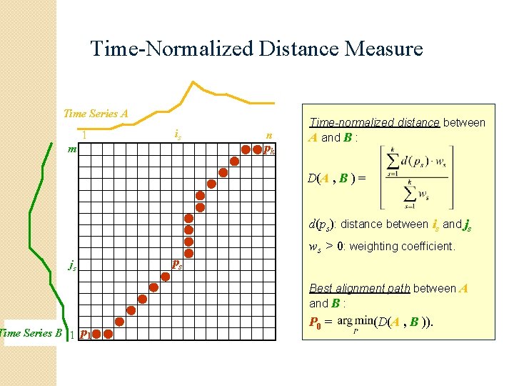
Time-Normalized Distance Measure Time Series A 1 is m n pk Time-normalized distance between A and B : D(A , B ) = d(ps): distance between is and js js Time Series B 1 ps ws > 0: weighting coefficient. Best alignment path between A and B : P 0 = (D(A , B )).

Matching words with DTW

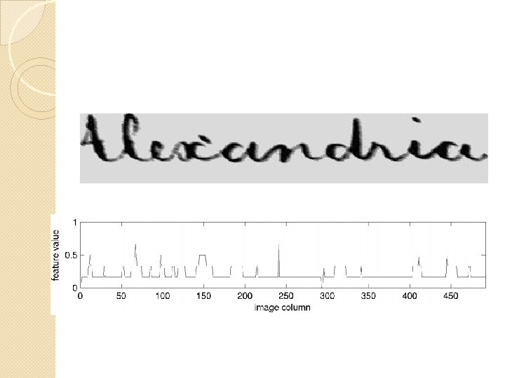
Matching words with DTW �The inter-character and intra-character spacing is subject to larger variations. �DTW offers a more flexible way compensate for these variations than linear scaling. �We first normalize the slant and skew angle of candidate images. �From each word, four features per image column are extracted and combined into a single time series.

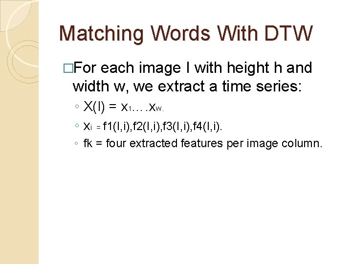
Matching Words With DTW �For each image I with height h and width w, we extract a time series: ◦ X(I) = x 1…. xw. ◦ xi = f 1(I, i), f 2(I, i), f 3(I, i), f 4(I, i). ◦ fk = four extracted features per image column.

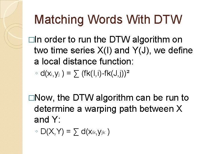
Matching Words With DTW �In order to run the DTW algorithm on two time series X(I) and Y(J), we define a local distance function: ◦ d(xi, yj ) = ∑ (fk(I, i)-fk(J, j))² �Now, the DTW algorithm can be run to determine a warping path between X and Y: ◦ D(X, Y) = ∑ d(xik, yjk )

DTW Features �Projection Profiles �Word Profiles ◦ Upper word profiles ◦ Lower word profiles �Background/Ink transitions

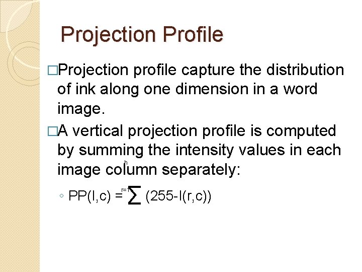
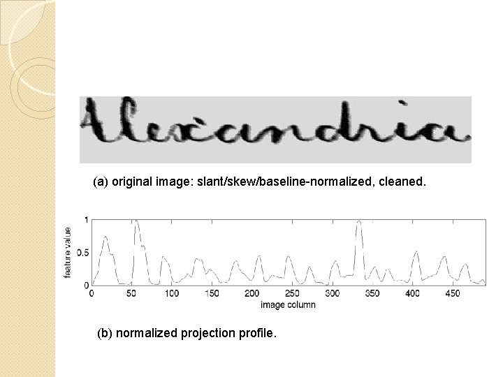
Projection Profile �Projection profile capture the distribution of ink along one dimension in a word image. �A vertical projection profile is computed by summing the intensity values in each image column separately: h ◦ PP(I, c) = ∑ (255 -I(r, c)) r=1

(a) original image: slant/skew/baseline-normalized, cleaned. (b) normalized projection profile.

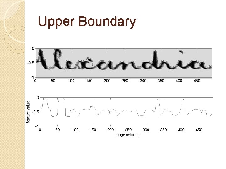
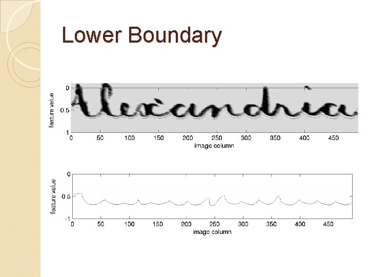
Word Profiles �Word profiles capture part of the outlining shape of a word. �Using upper and lower word profiles. �Going along the upper (lower) boundary of a word’s bounding box. �Recording for each image column the distance to the nearest “ink” pixel in that column.

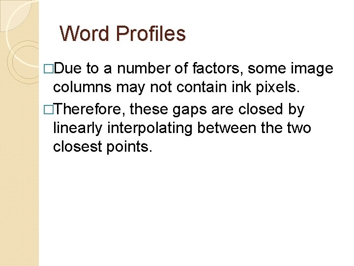
Word Profiles �Due to a number of factors, some image columns may not contain ink pixels. �Therefore, these gaps are closed by linearly interpolating between the two closest points.

Upper Boundary

Lower Boundary

Background/Ink Transitions �A capture of the inner structure of a word is missing. �Records for every image column, the number of transitions from the background to ink pixels: ◦ Determined by threshold. ◦ nbit(I, c).

Experimental Results �Data sets and processing �Results

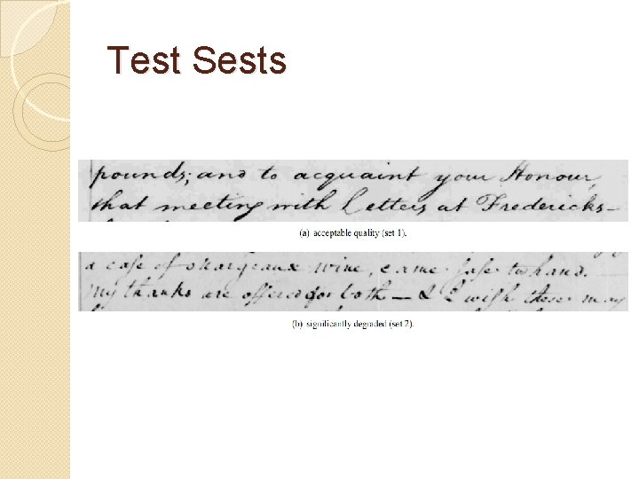
Data Sets And Processing �conducted on two test sets of different quality ◦ Acceptable quality (set 1). ◦ Very degraded quality (set 2). �Divide ◦ ◦ the test to four sets: 15 images in test set 1. Entire test set 1. 32 images in test set 2. Entire test set 2.

Test Sests

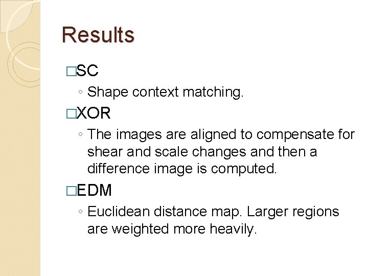
Results �SC ◦ Shape context matching. �XOR ◦ The images are aligned to compensate for shear and scale changes and then a difference image is computed. �EDM ◦ Euclidean distance map. Larger regions are weighted more heavily.

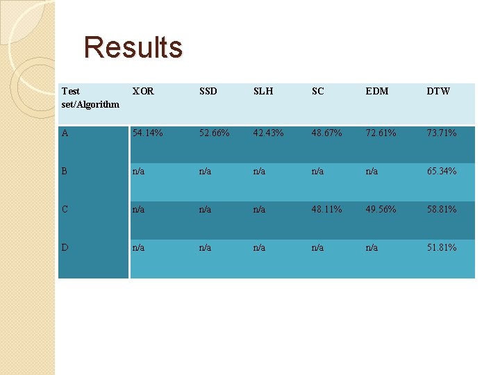
Results Test set/Algorithm XOR SSD SLH SC EDM DTW A 54. 14% 52. 66% 42. 43% 48. 67% 72. 61% 73. 71% B n/a n/a n/a 65. 34% C n/a n/a 48. 11% 49. 56% 58. 81% D n/a n/a n/a 51. 81%

Summary & Conclusions �DTW approach perform better than a number of other techniques. ◦ Accuracy. ◦ Speed. �The future work will focus on improvements in speed and accuracy. ◦ Pruning. ◦ Optimizations in DTW.