Word Sense Disambiguation Hsu TingWei Presented by Patty

Word Sense Disambiguation Hsu Ting-Wei Presented by Patty Liu

Outline • Introduction – 7. 1 Methodological Preliminaries • 7. 1. 1 Supervised and Unsupervised learning • 7. 1. 2 Pseudowords • 7. 1. 3 Upper and lower bounds on performance • Methods for Disambiguation – 7. 2 Supervised Disambiguation • 7. 2. 1 Bayesian classification • 7. 2. 2 An information-theoretic approach – 7. 3 Dictionary-based Disambiguation • 7. 3. 1 Disambiguation based on sense definitions • 7. 3. 2 Thesaurus-based disambiguation • 7. 3. 3 Disambiguation based on translations in a second-language corpus • 7. 3. 4 One sense per discourse, one sense per collocation – 7. 4 Unsupervised Disambiguation 2

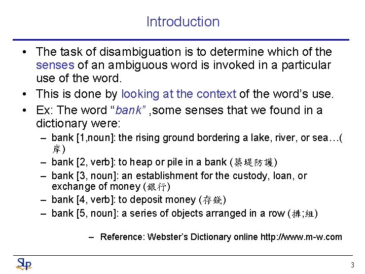
Introduction • The task of disambiguation is to determine which of the senses of an ambiguous word is invoked in a particular use of the word. • This is done by looking at the context of the word’s use. • Ex: The word “bank” , some senses that we found in a dictionary were: – bank [1, noun]: the rising ground bordering a lake, river, or sea…( 岸) – bank [2, verb]: to heap or pile in a bank (築堤防護) – bank [3, noun]: an establishment for the custody, loan, or exchange of money (銀行) – bank [4, verb]: to deposit money (存錢) – bank [5, noun]: a series of objects arranged in a row (排; 組) – Reference: Webster’s Dictionary online http: //www. m-w. com 3

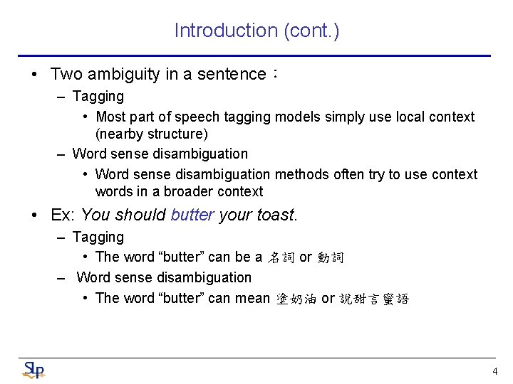
Introduction (cont. ) • Two ambiguity in a sentence： – Tagging • Most part of speech tagging models simply use local context (nearby structure) – Word sense disambiguation • Word sense disambiguation methods often try to use context words in a broader context • Ex: You should butter your toast. – Tagging • The word “butter” can be a 名詞 or 動詞 – Word sense disambiguation • The word “butter” can mean 塗奶油 or 說甜言蜜語 4

7. 1 Methodological Preliminaries • 7. 1. 1 Supervised and Unsupervised learning – Supervised learning (classification、function-fitting) • The actual status for each piece of data on which we train • One extrapolates the shape of a function based on some data points. – Unsupervised learning (clustering task) • We don’t know the classification of the data in the training sample 5

7. 1 Methodological Preliminaries (cont. ) • 7. 1. 2 Pseudowords – Hand-labeling is a time intensive and laborious task – Test data are hard to come by – It is often convenient to generate artificial evaluation data for the comparison and improvement of text procession algorithms – Artificial ambiguous words can be created by conflating two or more natural words – Ex: banana-door – Easy to create large-scale train/test set 6

7. 1 Methodological Preliminaries (cont. ) • 7. 1. 3 Upper and lower bounds on performance – It’s meaningless that only consider numerical evaluation • Need to consider how difficult the task is – Using upper and lower bounds to estimate • Upper bound human performance – We can’t expect an automatic procedure to do better • Lower bound (baseline) the simplest possible algorithm – Assignment of all contexts to the most frequent sense 7

Methods for Disambiguation • 7. 2 Supervised Disambiguation – Disambiguation based on a labeled training set • 7. 3 Dictionary-based – Disambiguation based on lexical resources such as dictionaries and thesauri • 7. 4 Unsupervised Disambiguation – Disambiguation based on training on an unlabeled text corpora. 8

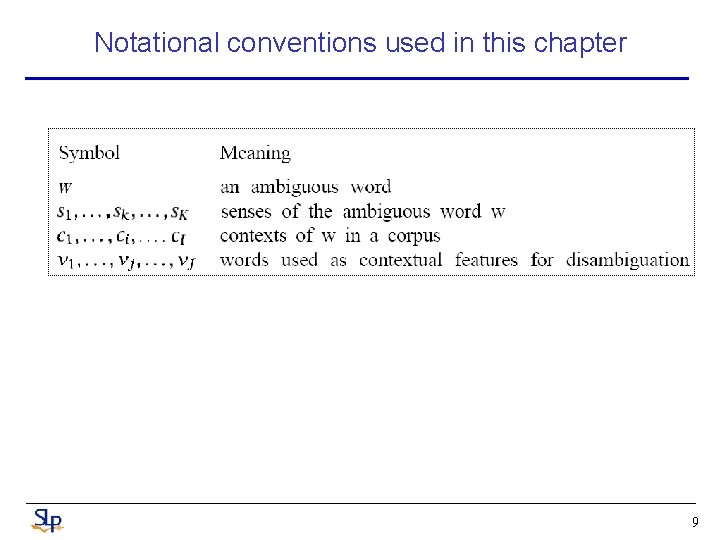
Notational conventions used in this chapter 9

7. 2 Supervised Disambiguation • Training corpus: Each occurrence of the ambiguous word w is annotated with a semantic label • Supervised disambiguation is a classification task. • We will look at: – Bayesian classification (Gale et al. 1992). – Information-theoretic approach (Brown et al. 1991) 10

7. 2 Supervised Disambiguation (cont. ) • 7. 2. 1 Bayesian classification (Gale et al. 1992) – The approach treats the context of occurrence as a bag of words without structure, but it integrates information from many words in the context window. (feature) – Bayes Decision rule • Decide s’ if P(s’ | c) > P(sk | c) for sk ≠s’ – Bayes decision rule is optimal because it minimizes the probability of error – Choose the class (or sense) with the highest conditional probability and hence the smallest error rate. 11

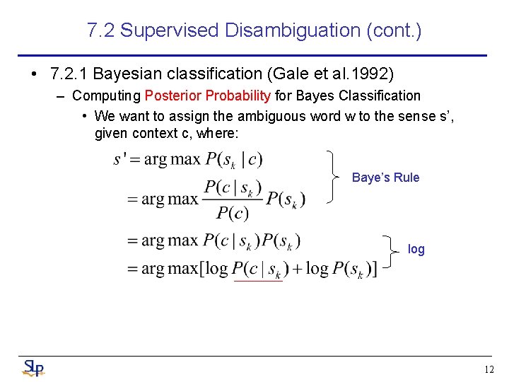
7. 2 Supervised Disambiguation (cont. ) • 7. 2. 1 Bayesian classification (Gale et al. 1992) – Computing Posterior Probability for Bayes Classification • We want to assign the ambiguous word w to the sense s’, given context c, where: Baye’s Rule log 12

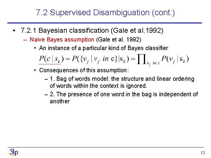
7. 2 Supervised Disambiguation (cont. ) • 7. 2. 1 Bayesian classification (Gale et al. 1992) – Naive Bayes assumption (Gale et al. 1992) • An instance of a particular kind of Bayes classifier • Consequences of this assumption: – 1. Bag of words model: the structure and linear ordering of words within the context is ignored. – 2. The presence of one word in the bag is independent of another 13

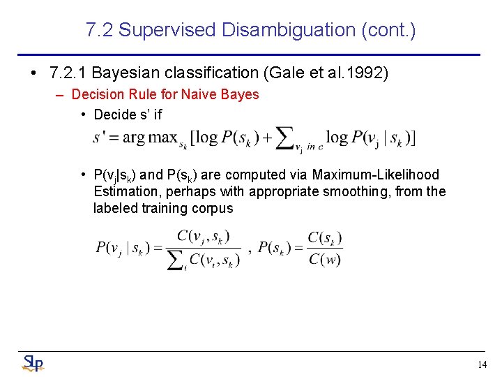
7. 2 Supervised Disambiguation (cont. ) • 7. 2. 1 Bayesian classification (Gale et al. 1992) – Decision Rule for Naive Bayes • Decide s’ if • P(vj|sk) and P(sk) are computed via Maximum-Likelihood Estimation, perhaps with appropriate smoothing, from the labeled training corpus 14

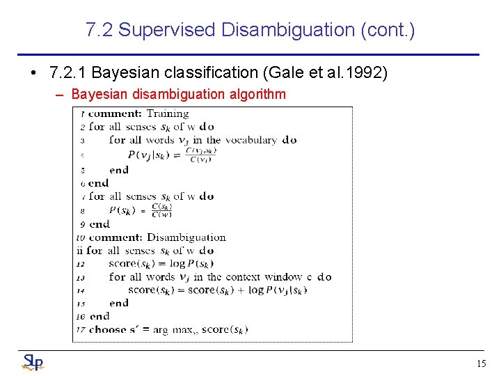
7. 2 Supervised Disambiguation (cont. ) • 7. 2. 1 Bayesian classification (Gale et al. 1992) – Bayesian disambiguation algorithm 15

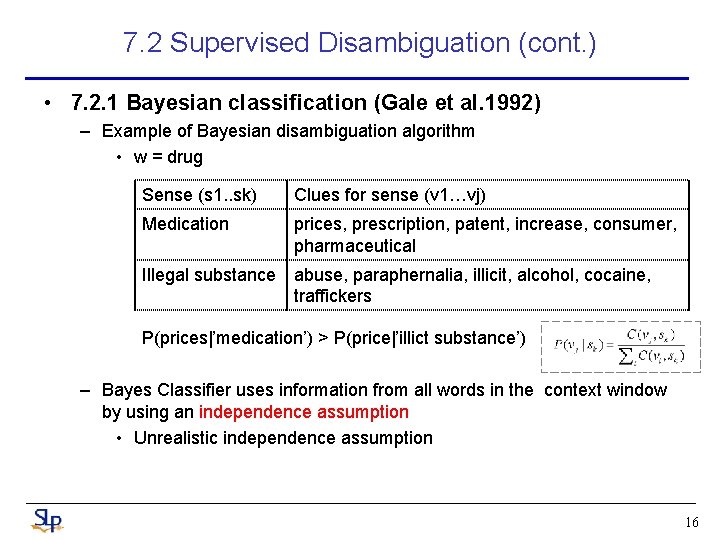
7. 2 Supervised Disambiguation (cont. ) • 7. 2. 1 Bayesian classification (Gale et al. 1992) – Example of Bayesian disambiguation algorithm • w = drug Sense (s 1. . sk) Clues for sense (v 1…vj) Medication prices, prescription, patent, increase, consumer, pharmaceutical Illegal substance abuse, paraphernalia, illicit, alcohol, cocaine, traffickers P(prices|’medication’) > P(price|’illict substance’) – Bayes Classifier uses information from all words in the context window by using an independence assumption • Unrealistic independence assumption 16

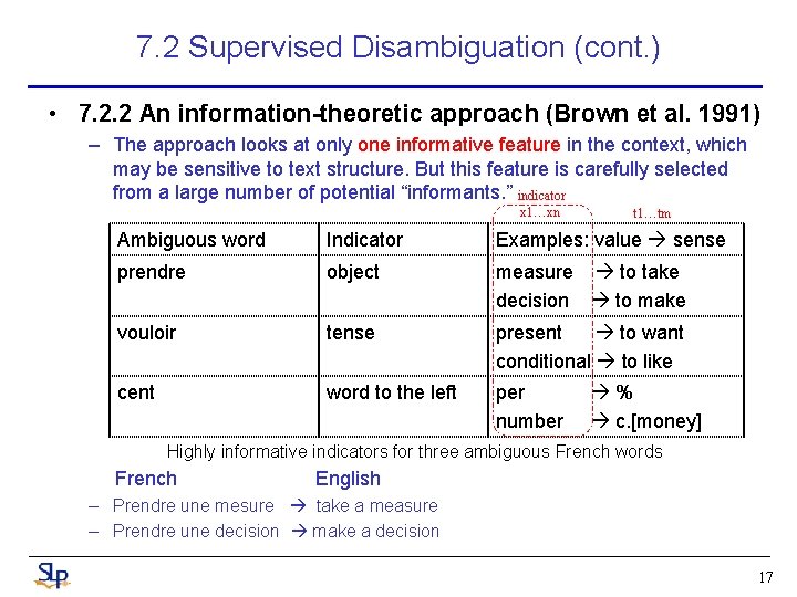
7. 2 Supervised Disambiguation (cont. ) • 7. 2. 2 An information-theoretic approach (Brown et al. 1991) – The approach looks at only one informative feature in the context, which may be sensitive to text structure. But this feature is carefully selected from a large number of potential “informants. ” indicator x 1…xn t 1…tm Ambiguous word Indicator Examples: value sense prendre object measure to take decision to make vouloir tense present to want conditional to like cent word to the left per number % c. [money] Highly informative indicators for three ambiguous French words French English – Prendre une mesure take a measure – Prendre une decision make a decision 17

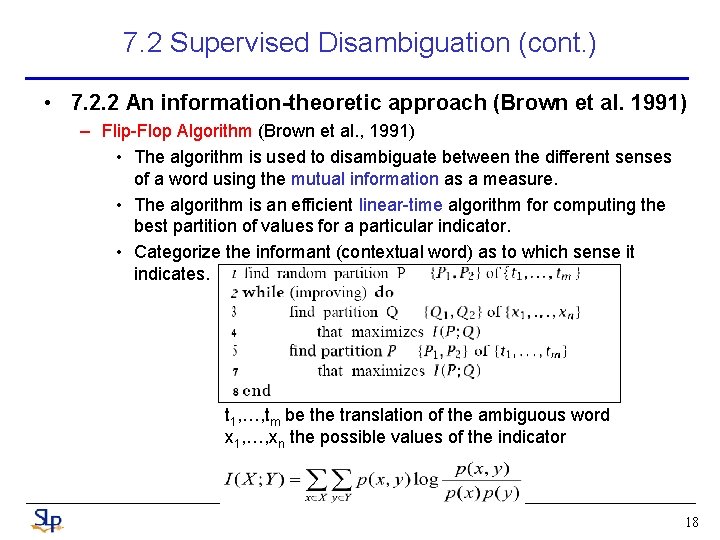
7. 2 Supervised Disambiguation (cont. ) • 7. 2. 2 An information-theoretic approach (Brown et al. 1991) – Flip-Flop Algorithm (Brown et al. , 1991) • The algorithm is used to disambiguate between the different senses of a word using the mutual information as a measure. • The algorithm is an efficient linear-time algorithm for computing the best partition of values for a particular indicator. • Categorize the informant (contextual word) as to which sense it indicates. t 1, …, tm be the translation of the ambiguous word x 1, …, xn the possible values of the indicator 18

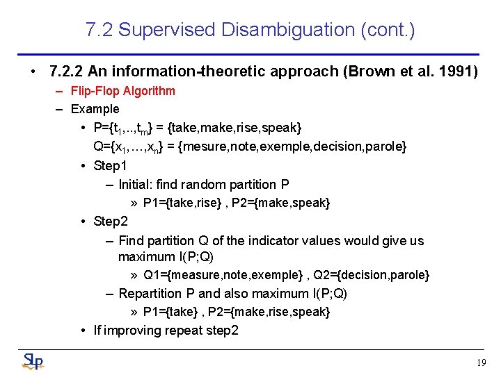
7. 2 Supervised Disambiguation (cont. ) • 7. 2. 2 An information-theoretic approach (Brown et al. 1991) – Flip-Flop Algorithm – Example • P={t 1, . . , tm} = {take, make, rise, speak} Q={x 1, …, xn} = {mesure, note, exemple, decision, parole} • Step 1 – Initial: find random partition P » P 1={take, rise} , P 2={make, speak} • Step 2 – Find partition Q of the indicator values would give us maximum I(P; Q) » Q 1={measure, note, exemple} , Q 2={decision, parole} – Repartition P and also maximum I(P; Q) » P 1={take} , P 2={make, rise, speak} • If improving repeat step 2 19

7. 3 Dictionary-based Disambiguation • If we have no information about the sense categorization of specific instance of a word, we can fall back on a general charaterization of the senses. • Sense definitions are extracted from existing sources such as dictionaries and thesaurus (類語詞典，表示一串有著相似、相關或相反意思的單字) • The different types of informational method have been used: – – 7. 3. 1 Disambiguation based on sense definitions 7. 3. 2 Thesaurus-based disambiguation 7. 3. 3 Disambiguation based on translations in a second-language corpus 7. 3. 4 One sense per discourse, one sense per collocation 20

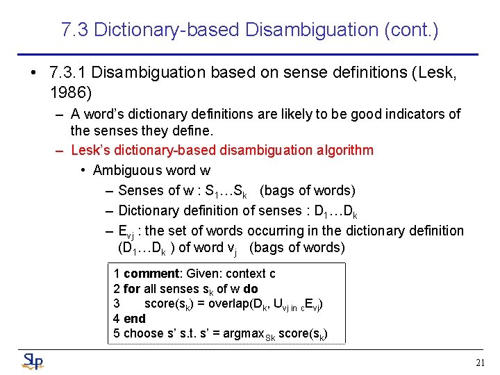
7. 3 Dictionary-based Disambiguation (cont. ) • 7. 3. 1 Disambiguation based on sense definitions (Lesk, 1986) – A word’s dictionary definitions are likely to be good indicators of the senses they define. – Lesk’s dictionary-based disambiguation algorithm • Ambiguous word w – Senses of w : S 1…Sk (bags of words) – Dictionary definition of senses : D 1…Dk – Evj : the set of words occurring in the dictionary definition (D 1…Dk ) of word vj (bags of words) 1 comment: Given: context c 2 for all senses sk of w do 3 score(sk) = overlap(Dk, Uvj in c. Evj) 4 end 5 choose s’ s. t. s’ = argmax. Sk score(sk) 21

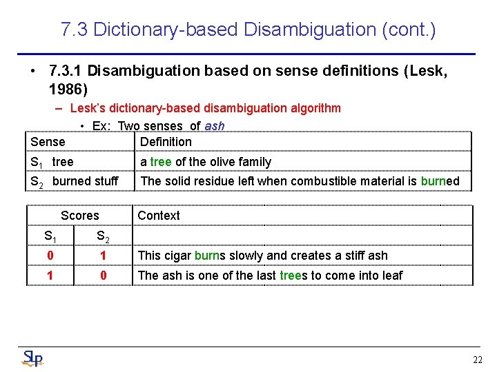
7. 3 Dictionary-based Disambiguation (cont. ) • 7. 3. 1 Disambiguation based on sense definitions (Lesk, 1986) – Lesk’s dictionary-based disambiguation algorithm • Ex: Two senses of ash Sense Definition S 1 tree a tree of the olive family S 2 burned stuff The solid residue left when combustible material is burned Scores Context S 1 S 2 0 1 This cigar burns slowly and creates a stiff ash 1 0 The ash is one of the last trees to come into leaf 22

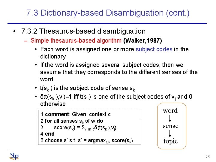
7. 3 Dictionary-based Disambiguation (cont. ) • 7. 3. 2 Thesaurus-based disambiguation – Simple thesaurus-based algorithm (Walker, 1987) • Each word is assigned one or more subject codes in the dictionary • If the word is assigned several subject codes, then we assume that they corresponds to the different senses of the word. • t(sk ) is the subject code of sense sk • δ(t(sk ), vj)=1 iff t(sk) is one of the subject codes of vj and 0 otherwise 1 comment: Given: context c 2 for all senses sk of w do 3 score(sk) = Σvj in cδ(t(sk ), vj) 4 end 5 choose s’ s. t. s’ = argmax. Sk score(sk) word sense topic 23

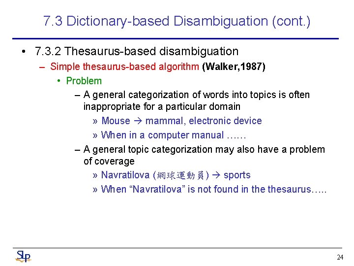
7. 3 Dictionary-based Disambiguation (cont. ) • 7. 3. 2 Thesaurus-based disambiguation – Simple thesaurus-based algorithm (Walker, 1987) • Problem – A general categorization of words into topics is often inappropriate for a particular domain » Mouse mammal, electronic device » When in a computer manual …… – A general topic categorization may also have a problem of coverage » Navratilova (網球運動員) sports » When “Navratilova” is not found in thesaurus…. . 24

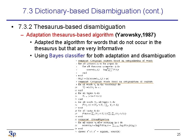
7. 3 Dictionary-based Disambiguation (cont. ) • 7. 3. 2 Thesaurus-based disambiguation – Adaptation thesaurus-based algorithm (Yarowsky, 1987) • Adapted the algorithm for words that do not occur in thesaurus but that are very Informative • Using Bayes classifier for both adaptation and disambiguation 25

7. 3 Dictionary-based Disambiguation (cont. ) • 7. 3. 3 Disambiguation based on translations in a secondlanguage corpus (Dagan et al. 1991; Dagan and Itai 1994) – Words can be disambiguated by looking at how they are translated in other languages – This method use of word correspondences in a bilingual dictionary • First Language – The one for which we want to disambiguation • Second Language – Target language in the bilingual dictionary – For example, if we want to disambiguate English based on German corpus, then English is the 1 st language, and the German is the 2 nd language. 26

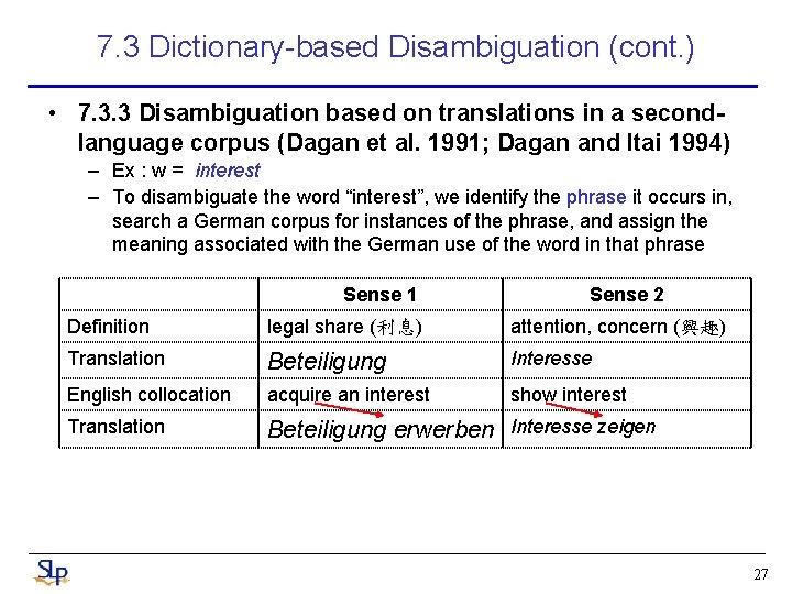
7. 3 Dictionary-based Disambiguation (cont. ) • 7. 3. 3 Disambiguation based on translations in a secondlanguage corpus (Dagan et al. 1991; Dagan and Itai 1994) – Ex : w = interest – To disambiguate the word “interest”, we identify the phrase it occurs in, search a German corpus for instances of the phrase, and assign the meaning associated with the German use of the word in that phrase Sense 1 Sense 2 Definition legal share (利息) attention, concern (興趣) Translation Beteiligung Interesse English collocation acquire an interest show interest Translation Beteiligung erwerben Interesse zeigen 27

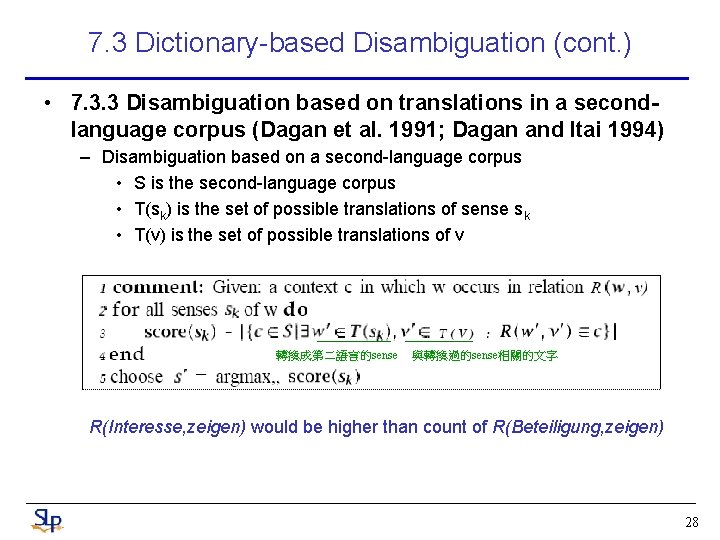
7. 3 Dictionary-based Disambiguation (cont. ) • 7. 3. 3 Disambiguation based on translations in a secondlanguage corpus (Dagan et al. 1991; Dagan and Itai 1994) – Disambiguation based on a second-language corpus • S is the second-language corpus • T(sk) is the set of possible translations of sense sk • T(v) is the set of possible translations of v 轉換成第二語言的sense 與轉換過的sense相關的文字 R(Interesse, zeigen) would be higher than count of R(Beteiligung, zeigen) 28

7. 3 Dictionary-based Disambiguation (cont. ) • 7. 3. 4 One sense per discourse, one sense per collocation (Yarowsky, 1995) – There are constraints between different occurrences of an ambiguous word within a corpus that can be exploited for disambiguation – One sense per discourse • The sense of a target word is highly consistent within any given document – One sense per collocation • Nearby words provide strong and consistent clues to the sense of a target word, conditional on relative distance, order and syntactic relationship 29

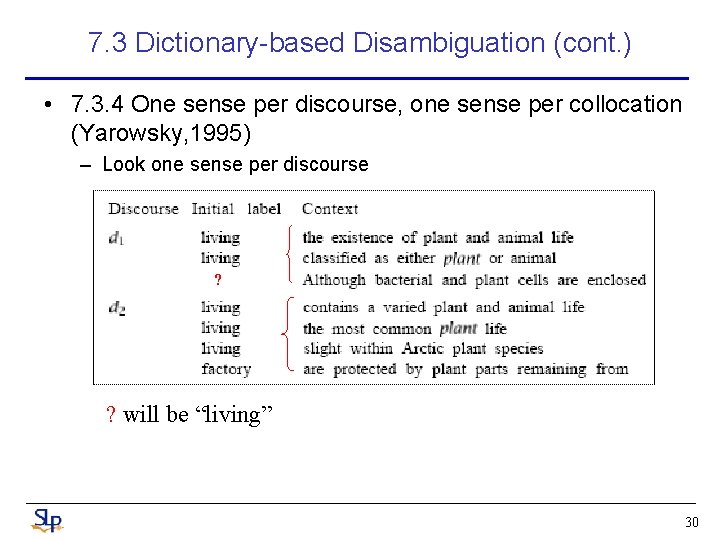
7. 3 Dictionary-based Disambiguation (cont. ) • 7. 3. 4 One sense per discourse, one sense per collocation (Yarowsky, 1995) – Look one sense per discourse ? ? will be “living” 30

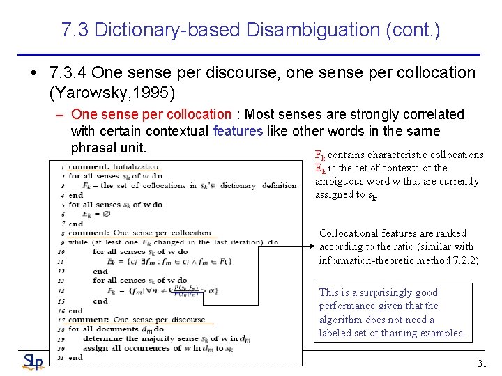
7. 3 Dictionary-based Disambiguation (cont. ) • 7. 3. 4 One sense per discourse, one sense per collocation (Yarowsky, 1995) – One sense per collocation : Most senses are strongly correlated with certain contextual features like other words in the same phrasal unit. F contains characteristic collocations. k Ek is the set of contexts of the ambiguous word w that are currently assigned to sk. Collocational features are ranked according to the ratio (similar with information-theoretic method 7. 2. 2) This is a surprisingly good performance given that the algorithm does not need a labeled set of thaining examples. 31

7. 4 Unsupervised Disambiguation • Cluster the contexts of an ambiguous word into a number of groups • Discriminate between these groups without labeling them – Probabilistic model is same the same with section 7. 2. 1 • Word : w • Senses : s 1…sk • Estimate P(vj|sk) , – In contrast to Gale et al. ’ s Bayes classifier, parameter estimation in unsupervised disambiguation is not based on a labeled training set. – Instead, we start with a random initialization of the parameters P(vj|sk). The P(vj|sk) are then reestimated by the EM algorithm. 32

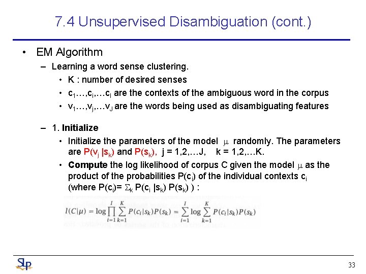
7. 4 Unsupervised Disambiguation (cont. ) • EM Algorithm – Learning a word sense clustering. • K : number of desired senses • c 1…, ci, …c. I are the contexts of the ambiguous word in the corpus • v 1…, vj, …v. J are the words being used as disambiguating features – 1. Initialize • Initialize the parameters of the model randomly. The parameters are P(vj |sk) and P(sk), j = 1, 2, …J, k = 1, 2, …K. • Compute the log likelihood of corpus C given the model as the product of the probabilities P(ci) of the individual contexts ci (where P(ci)= k P(ci |sk) P(sk) ) : 33

7. 4 Unsupervised Disambiguation (cont. ) • EM Algorithm – 2. While l(C| ) is improving repeat: • E-step: estimate hik , the posterior probability that sk generated ci, as follows: To compute P(ci|sk), we make the by now familiar Naïve Bayes assumption: • M-step: Re-estimate the parameters P(vj |sk) and P(sk) by way of maximum likelihood estimation: Recompute the probabilities of the senses as follows: 34

Thanks for your attention ! 35