Word classes and part of speech tagging Reading

Word classes and part of speech tagging Reading: Ch. 5, Jurafsky & Martin (Ch. 9 3 rd. Edition) PI Disclosure: This set includes adapted material from Rada Mihalcea, Raymond Mooney and Dan Jurafsky

Outline • • Review of coarse grammatical classes Why part of speech tagging? Tag sets and problem definition Automatic approaches: • HMMs • MEMMs 2

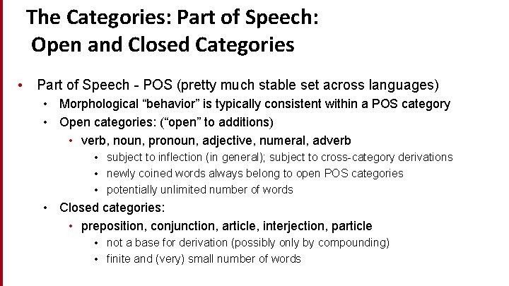
The Categories: Part of Speech: Open and Closed Categories • Part of Speech - POS (pretty much stable set across languages) • Morphological “behavior” is typically consistent within a POS category • Open categories: (“open” to additions) • verb, noun, pronoun, adjective, numeral, adverb • subject to inflection (in general); subject to cross-category derivations • newly coined words always belong to open POS categories • potentially unlimited number of words • Closed categories: • preposition, conjunction, article, interjection, particle • not a base for derivation (possibly only by compounding) • finite and (very) small number of words 3

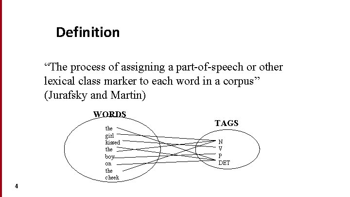
Definition “The process of assigning a part-of-speech or other lexical class marker to each word in a corpus” (Jurafsky and Martin) WORDS the girl kissed the boy on the cheek 4 TAGS N V P DET

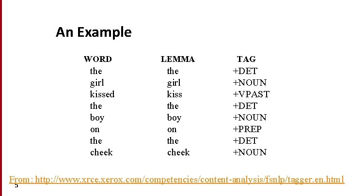
An Example WORD the girl kissed the boy on the cheek LEMMA the girl kiss the boy on the cheek TAG +DET +NOUN +VPAST +DET +NOUN +PREP +DET +NOUN From: http: //www. xrce. xerox. com/competencies/content-analysis/fsnlp/tagger. en. html 5

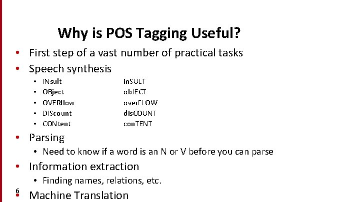
Why is POS Tagging Useful? • First step of a vast number of practical tasks • Speech synthesis • • • INsult OBject OVERflow DIScount CONtent in. SULT ob. JECT over. FLOW dis. COUNT con. TENT • Parsing • Need to know if a word is an N or V before you can parse • Information extraction • Finding names, relations, etc. 6 • Machine Translation

Outline • Why part of speech tagging? • Tag sets and problem definition • Automatic approaches: • HMMs • MEMMs 7

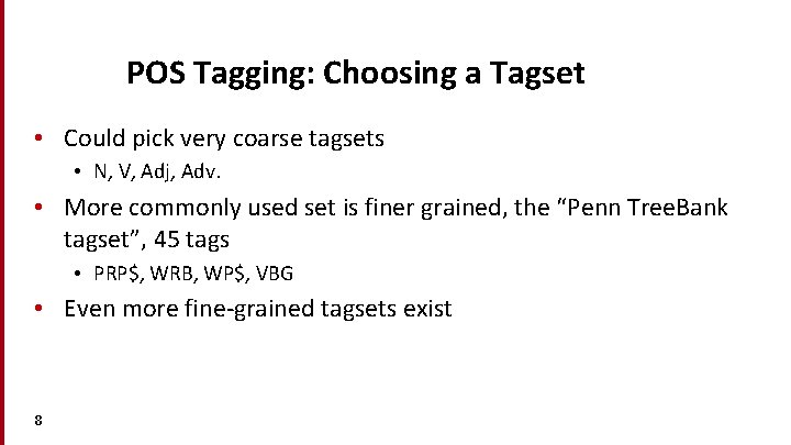
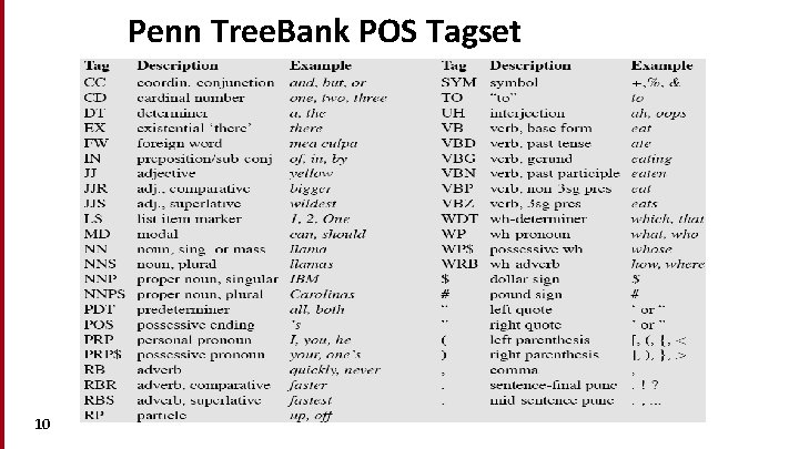
POS Tagging: Choosing a Tagset • Could pick very coarse tagsets • N, V, Adj, Adv. • More commonly used set is finer grained, the “Penn Tree. Bank tagset”, 45 tags • PRP$, WRB, WP$, VBG • Even more fine-grained tagsets exist 8

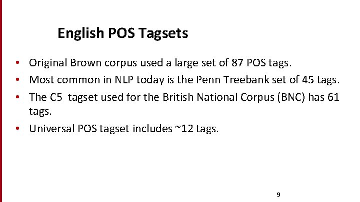
English POS Tagsets • Original Brown corpus used a large set of 87 POS tags. • Most common in NLP today is the Penn Treebank set of 45 tags. • The C 5 tagset used for the British National Corpus (BNC) has 61 tags. • Universal POS tagset includes ~12 tags. 9

Penn Tree. Bank POS Tagset 10

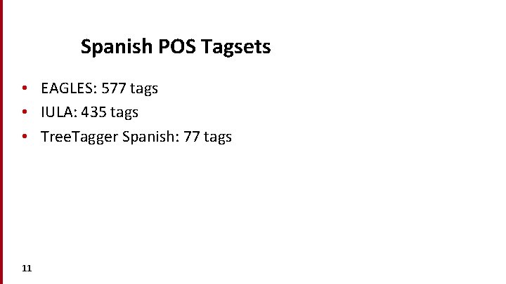
Spanish POS Tagsets • EAGLES: 577 tags • IULA: 435 tags • Tree. Tagger Spanish: 77 tags 11

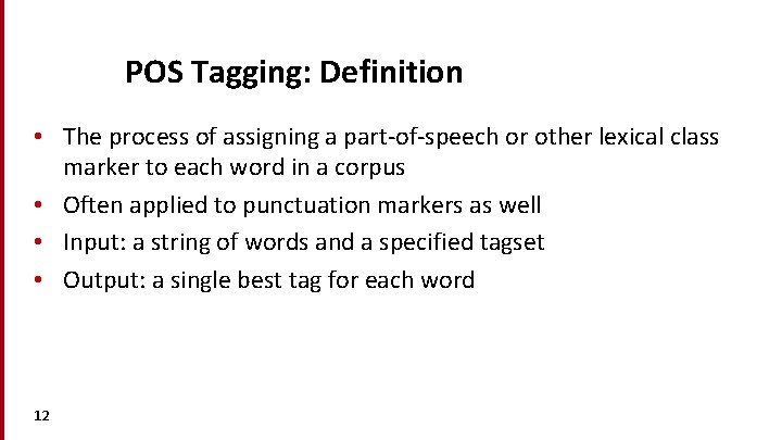
POS Tagging: Definition • The process of assigning a part-of-speech or other lexical class marker to each word in a corpus • Often applied to punctuation markers as well • Input: a string of words and a specified tagset • Output: a single best tag for each word 12

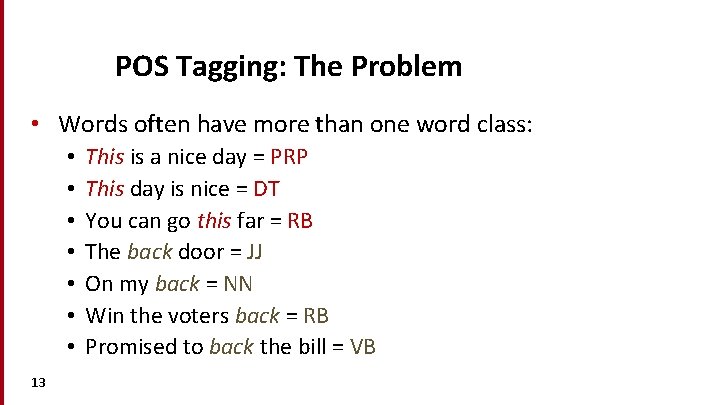
POS Tagging: The Problem • Words often have more than one word class: • • 13 This is a nice day = PRP This day is nice = DT You can go this far = RB The back door = JJ On my back = NN Win the voters back = RB Promised to back the bill = VB

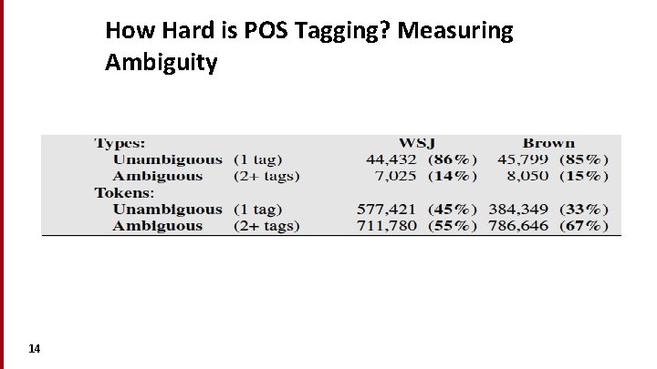
How Hard is POS Tagging? Measuring Ambiguity 14

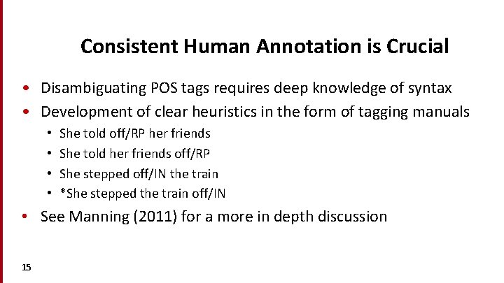
Consistent Human Annotation is Crucial • Disambiguating POS tags requires deep knowledge of syntax • Development of clear heuristics in the form of tagging manuals • • She told off/RP her friends She told her friends off/RP She stepped off/IN the train *She stepped the train off/IN • See Manning (2011) for a more in depth discussion 15

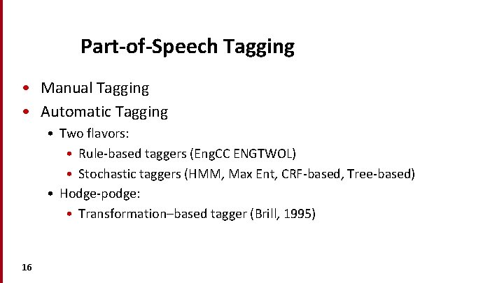
Part-of-Speech Tagging • Manual Tagging • Automatic Tagging • Two flavors: • Rule-based taggers (Eng. CC ENGTWOL) • Stochastic taggers (HMM, Max Ent, CRF-based, Tree-based) • Hodge-podge: • Transformation–based tagger (Brill, 1995) 16

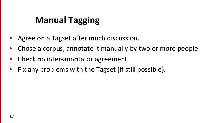
Manual Tagging • • 17 Agree on a Tagset after much discussion. Chose a corpus, annotate it manually by two or more people. Check on inter-annotator agreement. Fix any problems with the Tagset (if still possible).

Outline • Why part of speech tagging? • Tag sets and problem definition • Automatic approaches: • HMMs 18

Classification Learning • Typical machine learning addresses the problem of classifying a feature-vector description into a fixed number of classes. • There are many standard learning methods for this task: • • • 19 Decision Trees and Rule Learning Naïve Bayes and Bayesian Networks Logistic Regression / Maximum Entropy (Max. Ent) Perceptron and Neural Networks Support Vector Machines (SVMs) Nearest-Neighbor / Instance-Based

Beyond Classification Learning • Standard classification problem assumes individual cases are disconnected and independent. • Many NLP problems do not satisfy this assumption (involve many connected decisions, ambiguity and dependence) 20

Sequence Labeling Problem • Many NLP problems can be viewed as sequence labeling. • Each token in a sequence is assigned a label. • Labels of tokens are dependent on the labels of other tokens in the sequence, particularly their neighbors (not i. i. d). 21

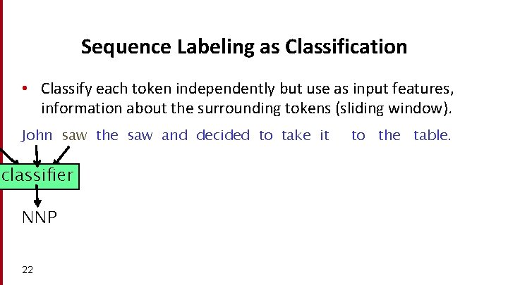
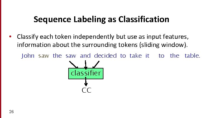
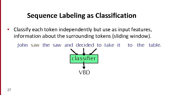
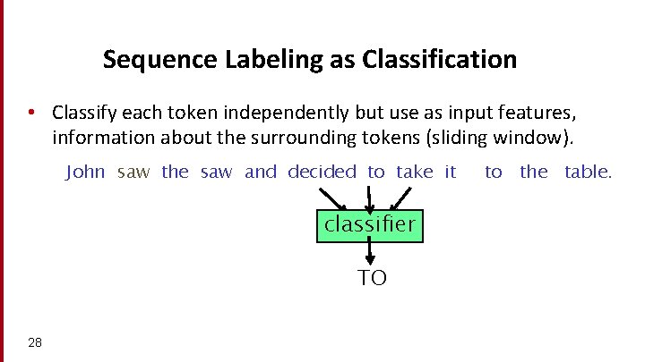
Sequence Labeling as Classification • Classify each token independently but use as input features, information about the surrounding tokens (sliding window). John saw the saw and decided to take it classifier NNP 22 to the table.

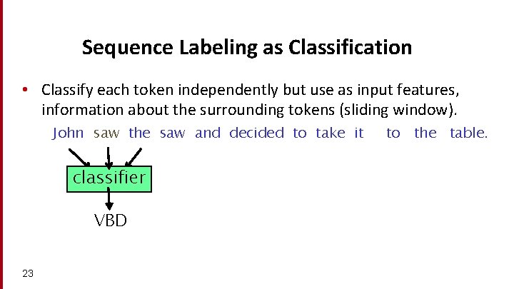
Sequence Labeling as Classification • Classify each token independently but use as input features, information about the surrounding tokens (sliding window). John saw the saw and decided to take it classifier VBD 23 to the table.

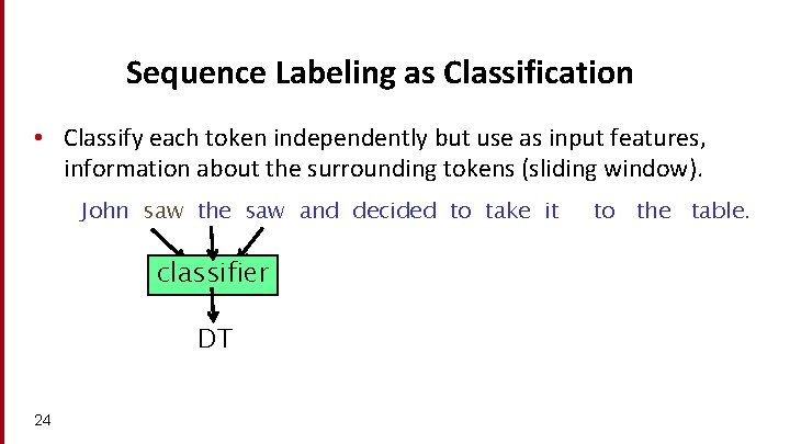
Sequence Labeling as Classification • Classify each token independently but use as input features, information about the surrounding tokens (sliding window). John saw the saw and decided to take it classifier DT 24 to the table.

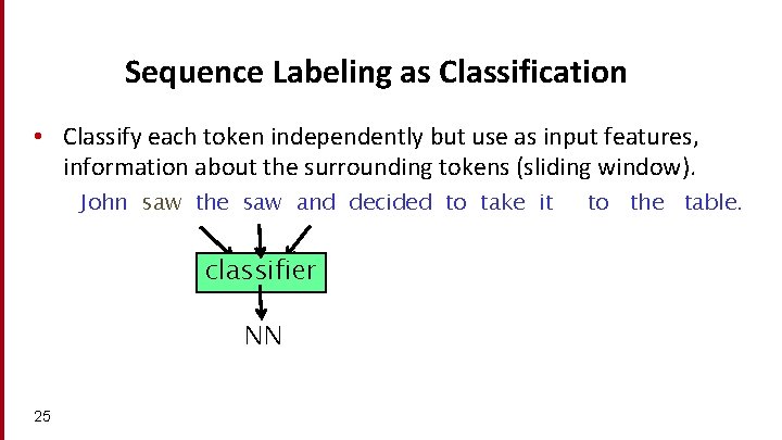
Sequence Labeling as Classification • Classify each token independently but use as input features, information about the surrounding tokens (sliding window). John saw the saw and decided to take it classifier NN 25 to the table.

Sequence Labeling as Classification • Classify each token independently but use as input features, information about the surrounding tokens (sliding window). John saw the saw and decided to take it classifier CC 26 to the table.

Sequence Labeling as Classification • Classify each token independently but use as input features, information about the surrounding tokens (sliding window). John saw the saw and decided to take it classifier VBD 27 to the table.

Sequence Labeling as Classification • Classify each token independently but use as input features, information about the surrounding tokens (sliding window). John saw the saw and decided to take it classifier TO 28 to the table.

Problems with Sequence Labeling as Classification • Not easy to integrate information from category of tokens on both sides. • Difficult to propagate uncertainty between decisions and “collectively” determine the most likely joint assignment of categories to all of the tokens in a sequence. 29

Probabilistic Sequence Models • Probabilistic sequence models allow interdependent classifications and collectively determine the most likely global assignment. • Two standard models • Hidden Markov Model (HMM) • Conditional Random Field (CRF) 30

POS Tagging as Sequence Classification • We are given a sentence (an “observation” or “sequence of observations”) • Secretariat is expected to race tomorrow • What is the best sequence of tags that corresponds to this sequence of observations? • Probabilistic view: • Consider all possible sequences of tags • Out of this universe of sequences, choose the tag sequence that is most probable given the observation sequence of n words w 1…wn. 31

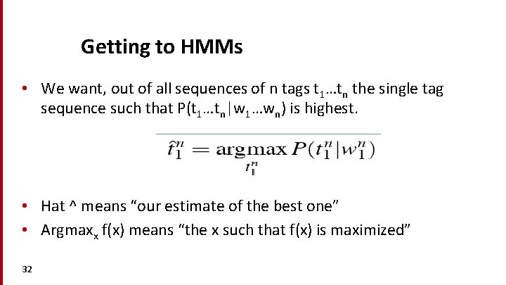
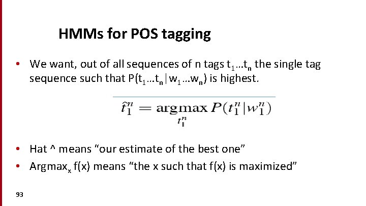
Getting to HMMs • We want, out of all sequences of n tags t 1…tn the single tag sequence such that P(t 1…tn|w 1…wn) is highest. • Hat ^ means “our estimate of the best one” • Argmaxx f(x) means “the x such that f(x) is maximized” 32

Hidden Markov Models

Outline • Introduction to Hidden Markov Models (HMMs) • Forward algorithm • Viterbi algorithm • Forward-Backward (Baum-Welch) 34

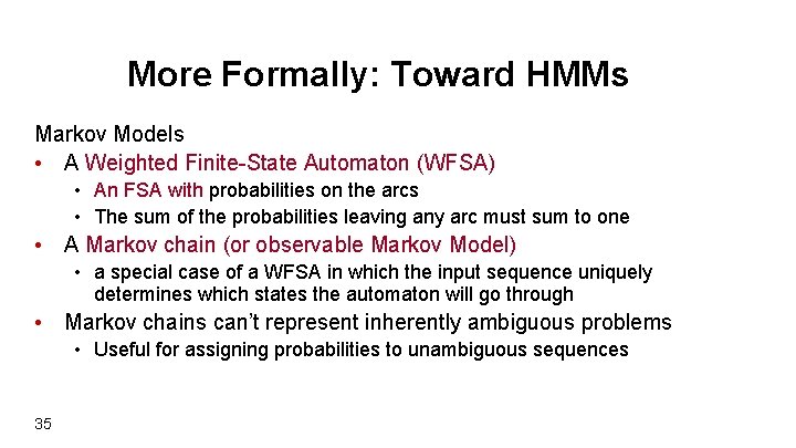
More Formally: Toward HMMs Markov Models • A Weighted Finite-State Automaton (WFSA) • An FSA with probabilities on the arcs • The sum of the probabilities leaving any arc must sum to one • A Markov chain (or observable Markov Model) • a special case of a WFSA in which the input sequence uniquely determines which states the automaton will go through • Markov chains can’t represent inherently ambiguous problems • Useful for assigning probabilities to unambiguous sequences 35

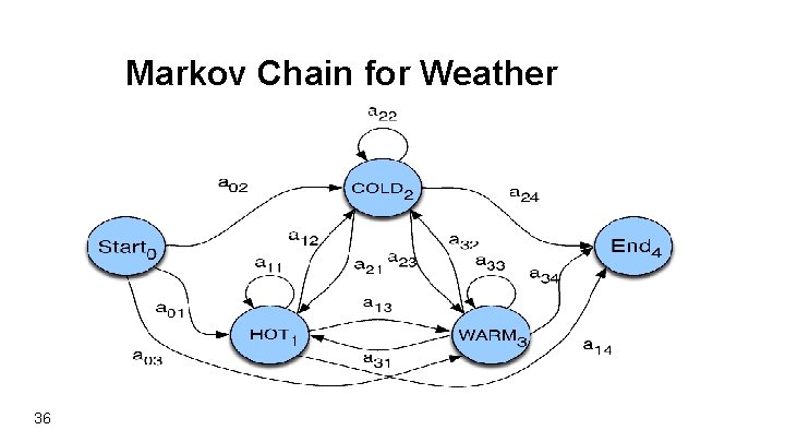
Markov Chain for Weather 36

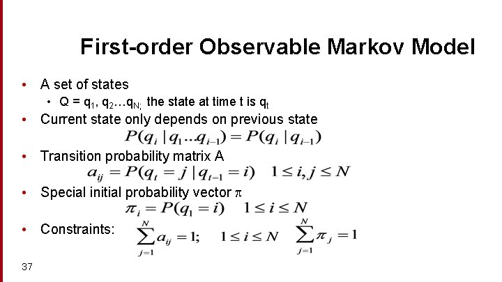
First-order Observable Markov Model • A set of states • Q = q 1, q 2…q. N; the state at time t is qt • Current state only depends on previous state • Transition probability matrix A • Special initial probability vector • Constraints: 37

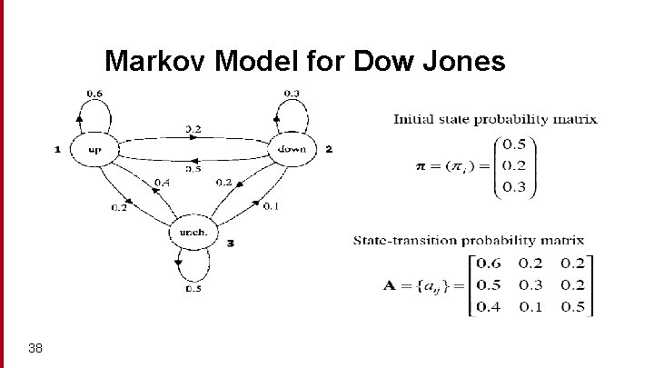
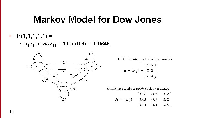
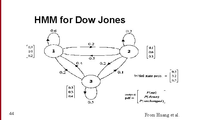
Markov Model for Dow Jones 38

Markov Model for Dow Jones • • 39 What is the probability of 5 consecutive up days? Sequence is up-up-up I. e. , state sequence is 1 -1 -1 P(1, 1, 1) = ?

Markov Model for Dow Jones • P(1, 1, 1) = • 1 a 11 a 11 = 0. 5 x (0. 6)4 = 0. 0648 40

Hidden Markov Model • For Markov chains, the output symbols are the same as the states • See up one day: we’re in state up • But in many NLP tasks: • output symbols are words • hidden states are something else • So we need an extension! • A Hidden Markov Model is an extension of a Markov chain in which the input symbols are not the same as the states. • This means we don’t know which state we are in. 41

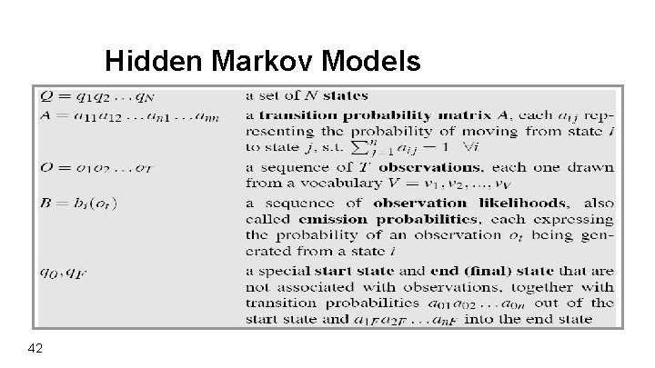
Hidden Markov Models 42

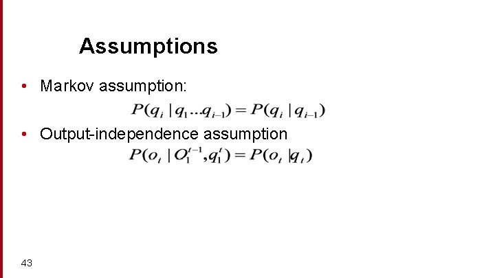
Assumptions • Markov assumption: • Output-independence assumption 43

HMM for Dow Jones 44 From Huang et al.

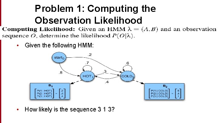
HMMs for Weather and Ice-cream • Jason Eisner’s cute HMM in Excel, showing Viterbi and EM: http: //www. cs. jhu. edu/~jason/papers/#teaching Idea: • You are climatologists in 3004 • Want to know about Baltimore weather in 2004 • Only data you have is Jason Eisner’s diary (how much ice cream he ate) • Observation: • Number of ice creams • Hidden State: Simplify to only 2 states • Weather is Hot or Cold that day. 45

The Three Basic Problems for HMMs • (From the classic formulation by Larry Rabiner after Jack Ferguson) • L. R. Rabiner. 1989. A tutorial on Hidden Markov Models and Selected Applications in Speech Recognition. Proc IEEE 77(2), 257 -286. Also in Waibel and Lee volume. 46

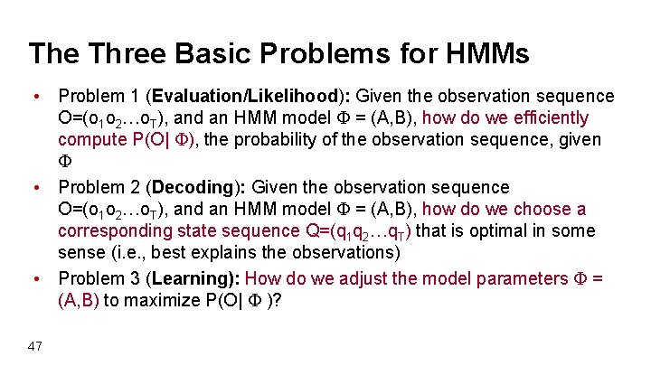
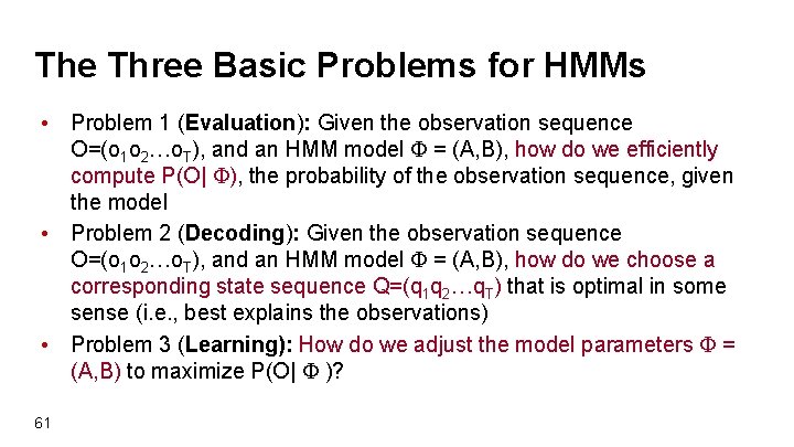
The Three Basic Problems for HMMs • Problem 1 (Evaluation/Likelihood): Given the observation sequence O=(o 1 o 2…o. T), and an HMM model = (A, B), how do we efficiently compute P(O| ), the probability of the observation sequence, given • Problem 2 (Decoding): Given the observation sequence O=(o 1 o 2…o. T), and an HMM model = (A, B), how do we choose a corresponding state sequence Q=(q 1 q 2…q. T) that is optimal in some sense (i. e. , best explains the observations) • Problem 3 (Learning): How do we adjust the model parameters = (A, B) to maximize P(O| )? 47

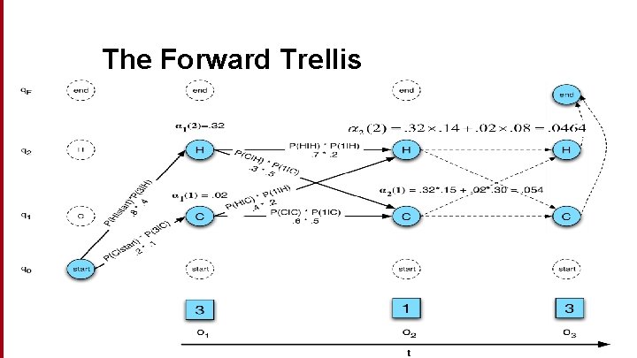
Problem 1: Computing the Observation Likelihood • Given the following HMM: • How likely is the sequence 3 1 3?

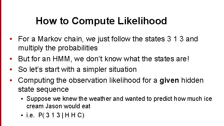
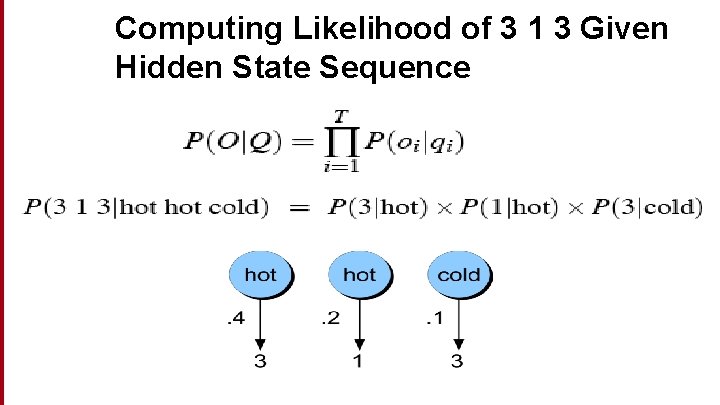
How to Compute Likelihood • For a Markov chain, we just follow the states 3 1 3 and multiply the probabilities • But for an HMM, we don’t know what the states are! • So let’s start with a simpler situation • Computing the observation likelihood for a given hidden state sequence • Suppose we knew the weather and wanted to predict how much ice cream Jason would eat • i. e. P( 3 1 3 | H H C)

Computing Likelihood of 3 1 3 Given Hidden State Sequence

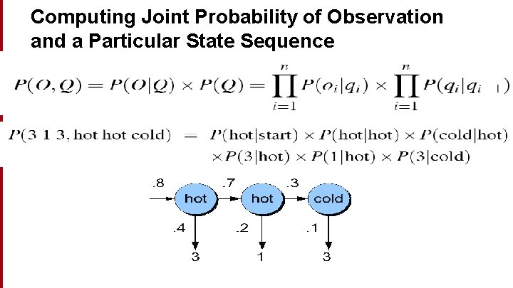
Computing Joint Probability of Observation and a Particular State Sequence

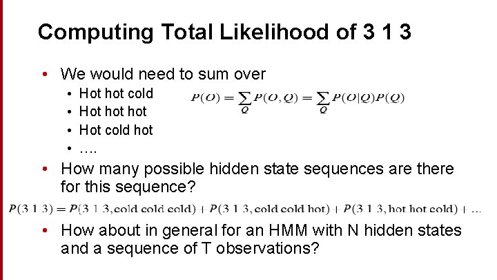
Computing Total Likelihood of 3 1 3 • We would need to sum over • • Hot hot cold Hot hot Hot cold hot …. • How many possible hidden state sequences are there for this sequence? • How about in general for an HMM with N hidden states and a sequence of T observations?

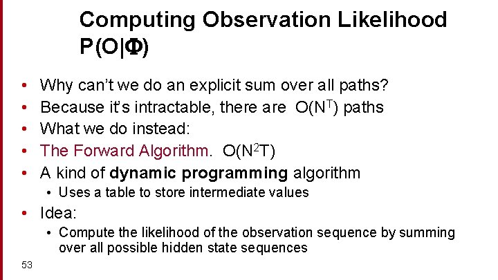
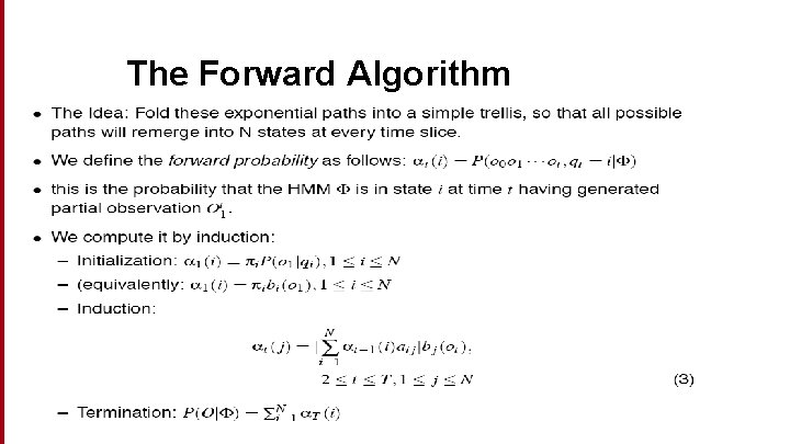
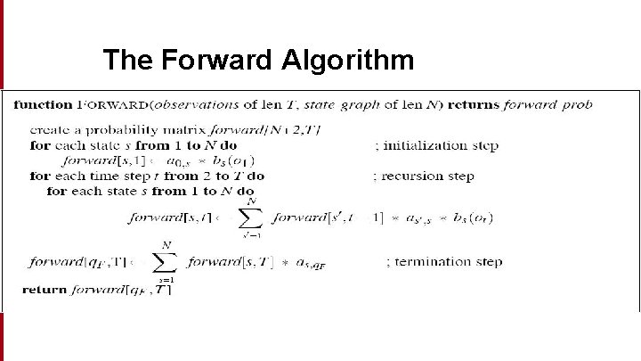
Computing Observation Likelihood P(O| ) • • • Why can’t we do an explicit sum over all paths? Because it’s intractable, there are O(NT) paths What we do instead: The Forward Algorithm. O(N 2 T) A kind of dynamic programming algorithm • Uses a table to store intermediate values • Idea: • Compute the likelihood of the observation sequence by summing over all possible hidden state sequences 53

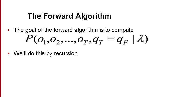
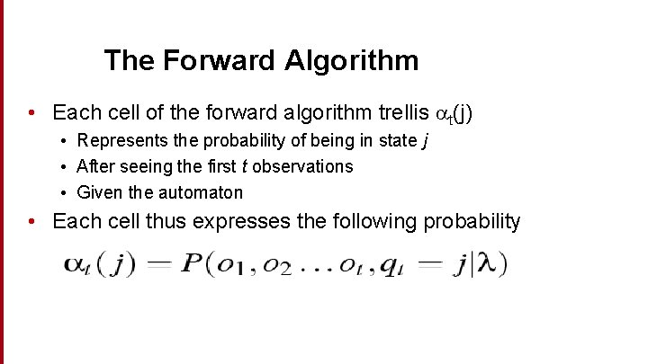
The Forward Algorithm • The goal of the forward algorithm is to compute • We’ll do this by recursion

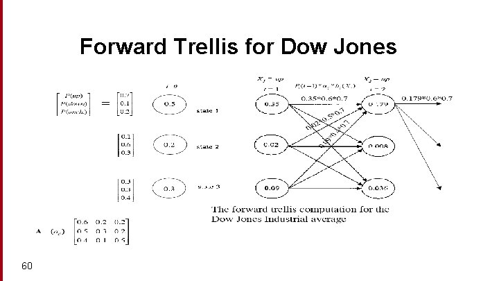
The Forward Algorithm • Each cell of the forward algorithm trellis t(j) • Represents the probability of being in state j • After seeing the first t observations • Given the automaton • Each cell thus expresses the following probability

The Forward Trellis

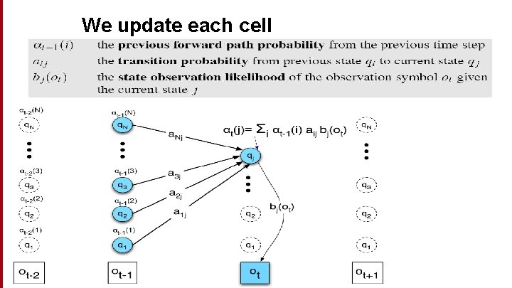
We update each cell

The Forward Algorithm 582006

The Forward Algorithm

Forward Trellis for Dow Jones 60

The Three Basic Problems for HMMs • Problem 1 (Evaluation): Given the observation sequence O=(o 1 o 2…o. T), and an HMM model = (A, B), how do we efficiently compute P(O| ), the probability of the observation sequence, given the model • Problem 2 (Decoding): Given the observation sequence O=(o 1 o 2…o. T), and an HMM model = (A, B), how do we choose a corresponding state sequence Q=(q 1 q 2…q. T) that is optimal in some sense (i. e. , best explains the observations) • Problem 3 (Learning): How do we adjust the model parameters = (A, B) to maximize P(O| )? 61

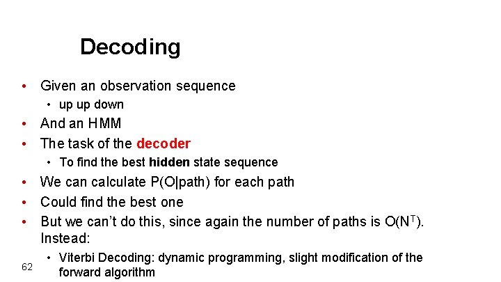
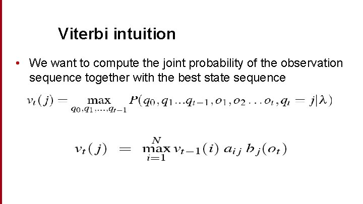
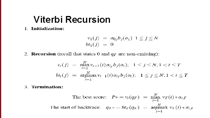
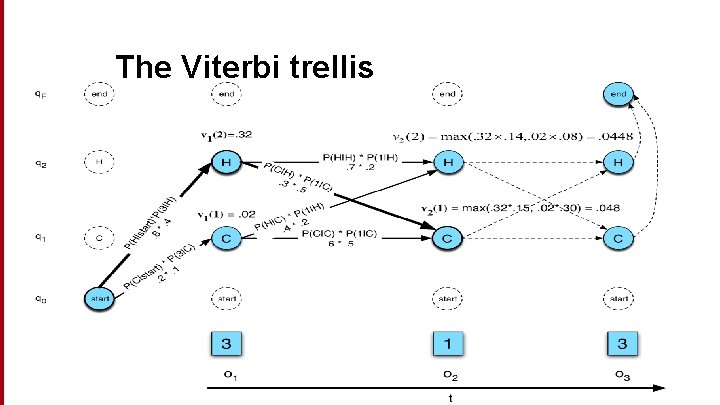
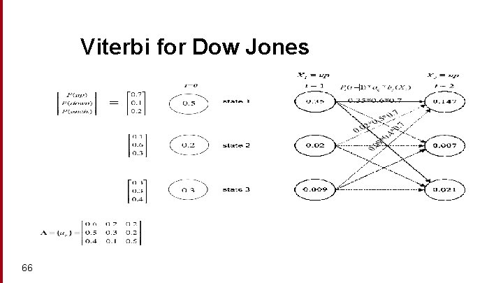
Decoding • Given an observation sequence • up up down • And an HMM • The task of the decoder • To find the best hidden state sequence • We can calculate P(O|path) for each path • Could find the best one • But we can’t do this, since again the number of paths is O(NT). Instead: 62 • Viterbi Decoding: dynamic programming, slight modification of the forward algorithm

Viterbi intuition • We want to compute the joint probability of the observation sequence together with the best state sequence

Viterbi Recursion

The Viterbi trellis

Viterbi for Dow Jones 66

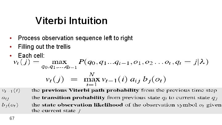
Viterbi Intuition • Process observation sequence left to right • Filling out the trellis • Each cell: 67

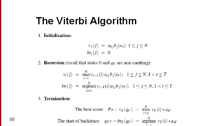
The Viterbi Algorithm 68

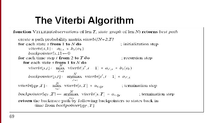
The Viterbi Algorithm 69

So Far… • Forward algorithm for evaluation • Viterbi algorithm for decoding • Next topic: the learning problem 70

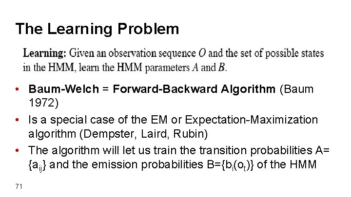
The Learning Problem • Baum-Welch = Forward-Backward Algorithm (Baum 1972) • Is a special case of the EM or Expectation-Maximization algorithm (Dempster, Laird, Rubin) • The algorithm will let us train the transition probabilities A= {aij} and the emission probabilities B={bi(ot)} of the HMM 71

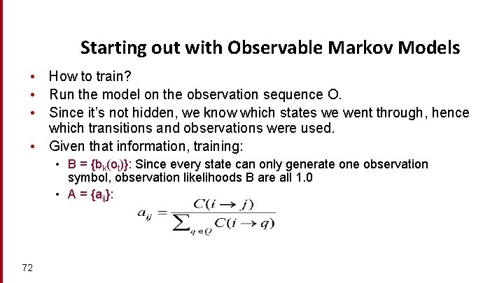
Starting out with Observable Markov Models • How to train? • Run the model on the observation sequence O. • Since it’s not hidden, we know which states we went through, hence which transitions and observations were used. • Given that information, training: • B = {bk(ot)}: Since every state can only generate one observation symbol, observation likelihoods B are all 1. 0 • A = {aij}: 72

Extending Intuition to HMMs • For HMMs, cannot compute these counts directly from observed sequences • Baum-Welch (forward-backward) intuitions: 73 • Iteratively estimate the counts • Start with an estimate for aij and bk, iteratively improve the estimates • Get estimated probabilities by: • computing the forward probability for an observation • dividing that probability mass among all the different paths that contributed to this forward probability • Two related probabilities: the forward probability and the backward probability

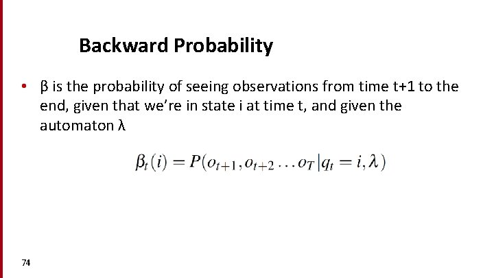
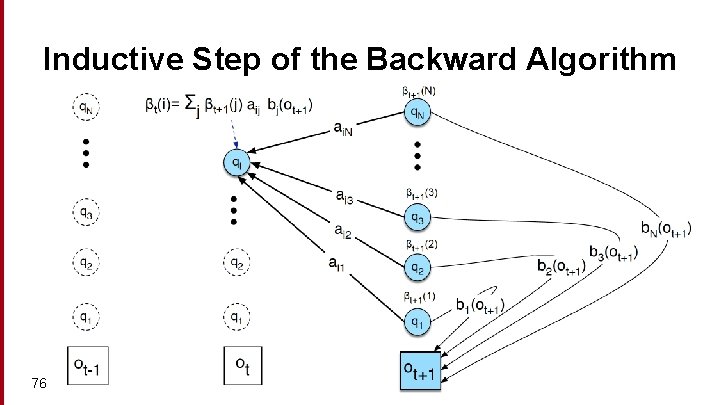
Backward Probability • β is the probability of seeing observations from time t+1 to the end, given that we’re in state i at time t, and given the automaton λ 74

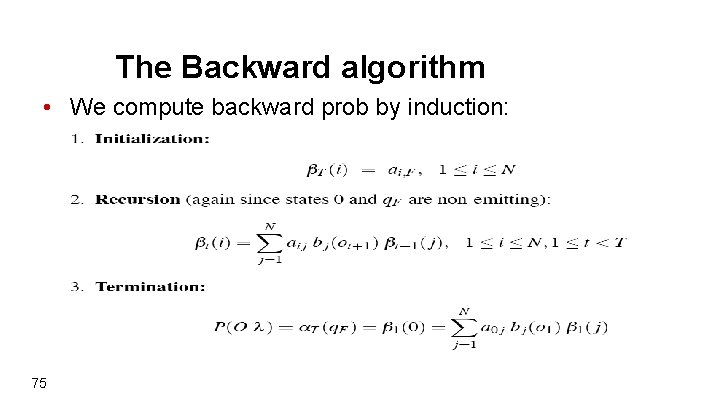
The Backward algorithm • We compute backward prob by induction: 75

Inductive Step of the Backward Algorithm 76

Extending Intuition to HMMs • For HMMs, cannot compute these counts directly from observed sequences • Baum-Welch (forward-backward) intuitions: 77 • Iteratively estimate the counts • Start with an estimate for aij and bk, iteratively improve the estimates • Get estimated probabilities by: • computing the forward probability for an observation • dividing that probability mass among all the different paths that contributed to this forward probability • Two related probabilities: the forward probability and the backward probability

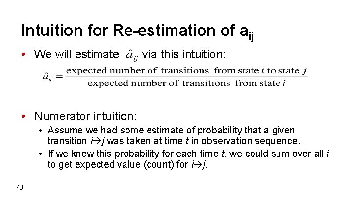
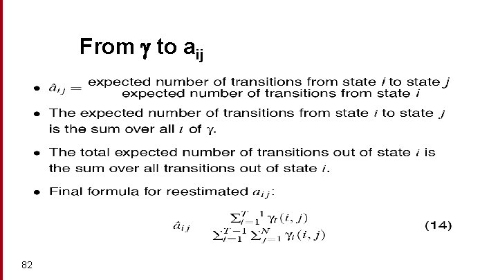
Intuition for Re-estimation of aij • We will estimate via this intuition: • Numerator intuition: • Assume we had some estimate of probability that a given transition i j was taken at time t in observation sequence. • If we knew this probability for each time t, we could sum over all t to get expected value (count) for i j. 78

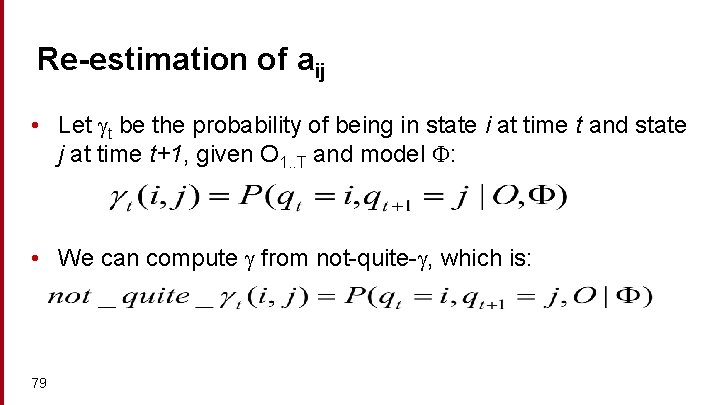
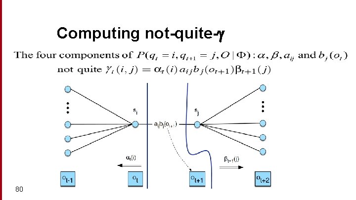
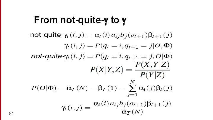
Re-estimation of aij • Let t be the probability of being in state i at time t and state j at time t+1, given O 1. . T and model : • We can compute from not-quite- , which is: 79

Computing not-quite- 80

From not-quite- to 81

From to aij 82

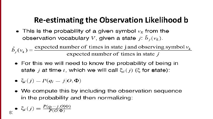
Re-estimating the Observation Likelihood b 83

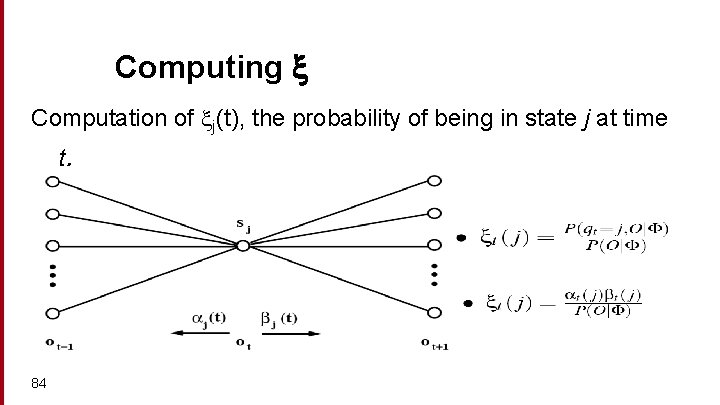
Computing Computation of j(t), the probability of being in state j at time t. 84

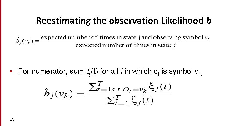
Reestimating the observation Likelihood b • For numerator, sum j(t) for all t in which ot is symbol vk: 85

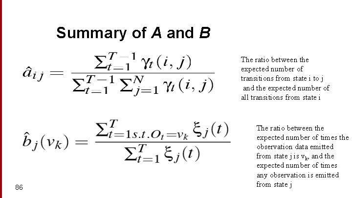
Summary of A and B The ratio between the expected number of transitions from state i to j and the expected number of all transitions from state i 86 The ratio between the expected number of times the observation data emitted from state j is vk, and the expected number of times any observation is emitted from state j

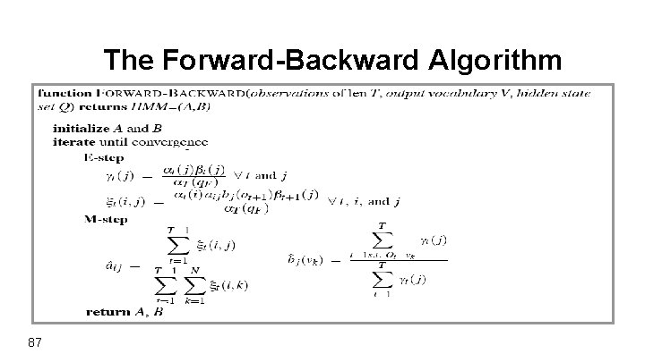
The Forward-Backward Algorithm 87

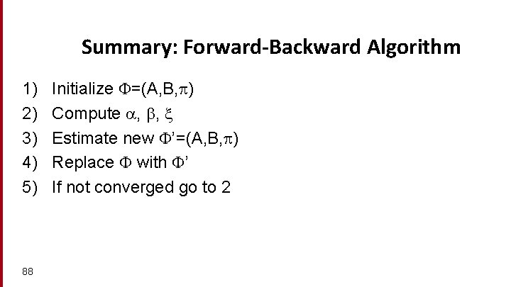
Summary: Forward-Backward Algorithm 1) 2) 3) 4) 5) 88 Initialize =(A, B, ) Compute , , Estimate new ’=(A, B, ) Replace with ’ If not converged go to 2

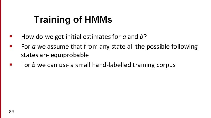
Training of HMMs § § § 89 How do we get initial estimates for a and b? For a we assume that from any state all the possible following states are equiprobable For b we can use a small hand-labelled training corpus

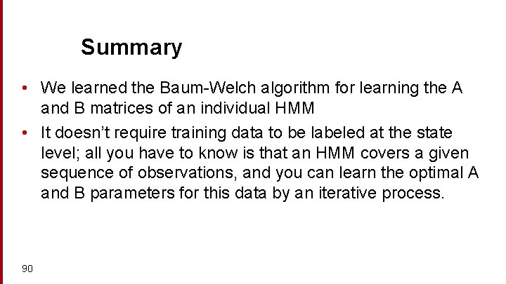
Summary • We learned the Baum-Welch algorithm for learning the A and B matrices of an individual HMM • It doesn’t require training data to be labeled at the state level; all you have to know is that an HMM covers a given sequence of observations, and you can learn the optimal A and B parameters for this data by an iterative process. 90

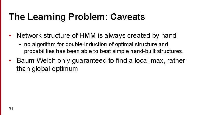
The Learning Problem: Caveats • Network structure of HMM is always created by hand • no algorithm for double-induction of optimal structure and probabilities has been able to beat simple hand-built structures. • Baum-Welch only guaranteed to find a local max, rather than global optimum 91

Now going back to POS tagging …

HMMs for POS tagging • We want, out of all sequences of n tags t 1…tn the single tag sequence such that P(t 1…tn|w 1…wn) is highest. • Hat ^ means “our estimate of the best one” • Argmaxx f(x) means “the x such that f(x) is maximized” 93

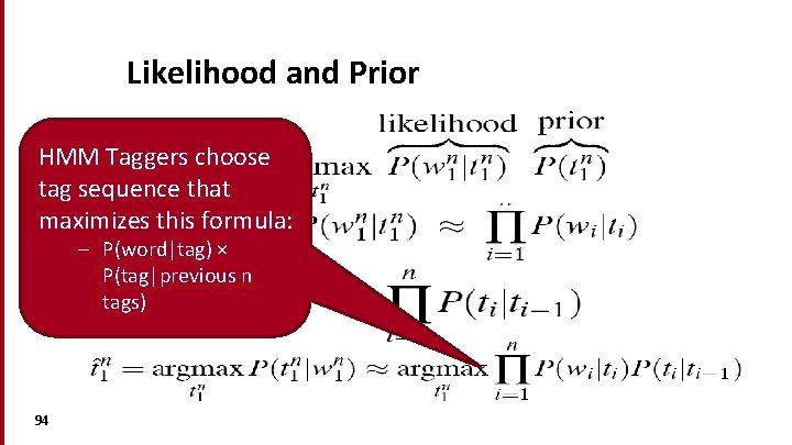
Likelihood and Prior HMM Taggers choose tag sequence that maximizes this formula: – P(word|tag) × P(tag|previous n tags) 94

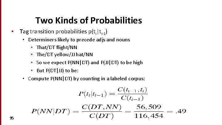
Two Kinds of Probabilities • Tag transition probabilities p(ti|ti-1) • Determiners likely to precede adjs and nouns • That/DT flight/NN • The/DT yellow/JJ hat/NN • So we expect P(NN|DT) and P(JJ|DT) to be high • But P(DT|JJ) to be: • Compute P(NN|DT) by counting in a labeled corpus: 95

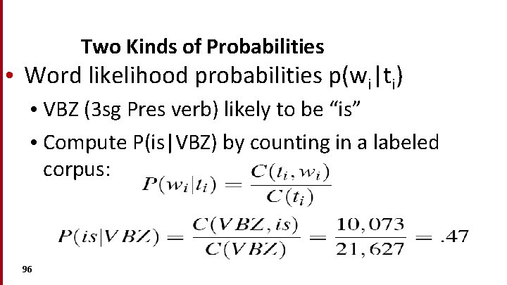
Two Kinds of Probabilities • Word likelihood probabilities p(wi|ti) • VBZ (3 sg Pres verb) likely to be “is” • Compute P(is|VBZ) by counting in a labeled corpus: 96

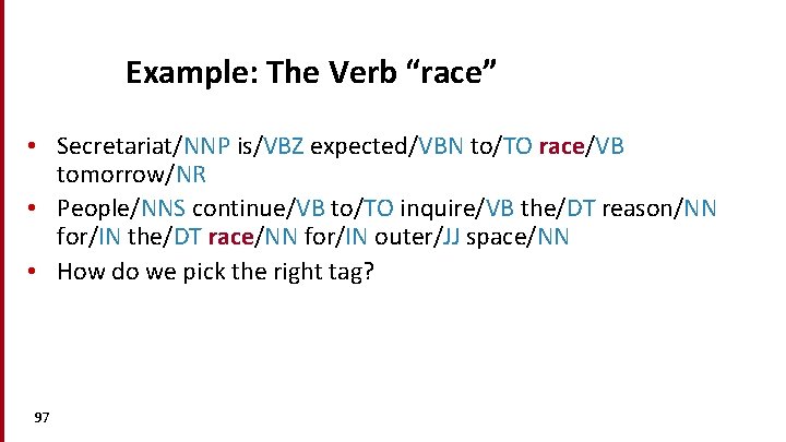
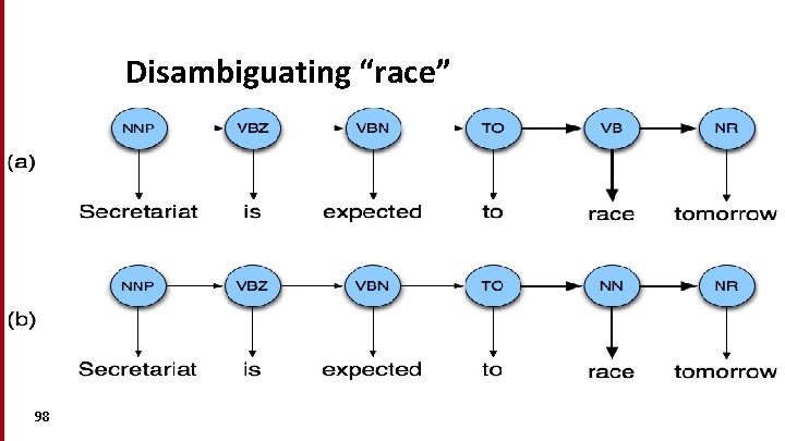
Example: The Verb “race” • Secretariat/NNP is/VBZ expected/VBN to/TO race/VB tomorrow/NR • People/NNS continue/VB to/TO inquire/VB the/DT reason/NN for/IN the/DT race/NN for/IN outer/JJ space/NN • How do we pick the right tag? 97

Disambiguating “race” 98

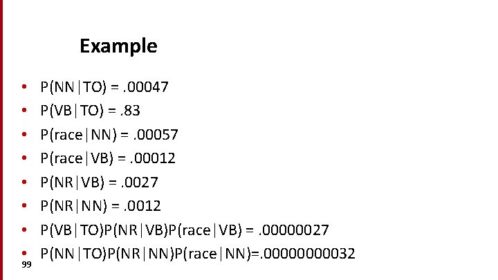
Example • • 99 P(NN|TO) =. 00047 P(VB|TO) =. 83 P(race|NN) =. 00057 P(race|VB) =. 00012 P(NR|VB) =. 0027 P(NR|NN) =. 0012 P(VB|TO)P(NR|VB)P(race|VB) =. 00000027 P(NN|TO)P(NR|NN)P(race|NN)=. 0000032

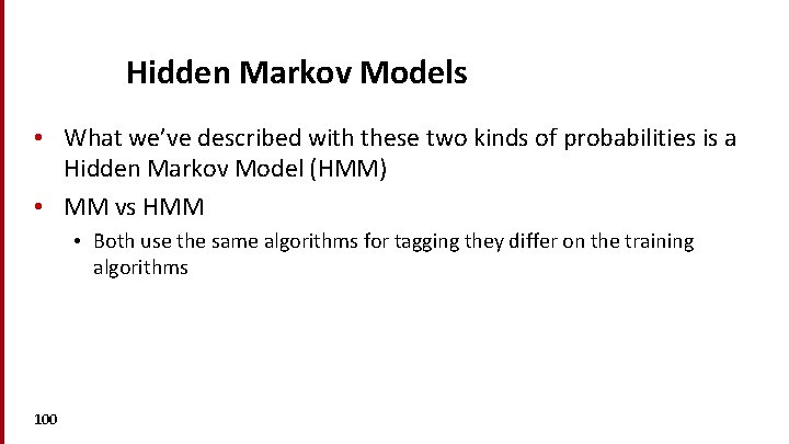
Hidden Markov Models • What we’ve described with these two kinds of probabilities is a Hidden Markov Model (HMM) • MM vs HMM • Both use the same algorithms for tagging they differ on the training algorithms 100

Example animation 101

An Early Approach to Statistical POS Tagging • PARTS tagger (Church, 1988): Stores probability of tag given word instead of word given tag. • P(tag|word) × P(tag|previous n tags) • Compare to: – P(word|tag) × P(tag|previous n tags) • What is the main difference between PARTS tagger (Church) and the HMM tagger? 102

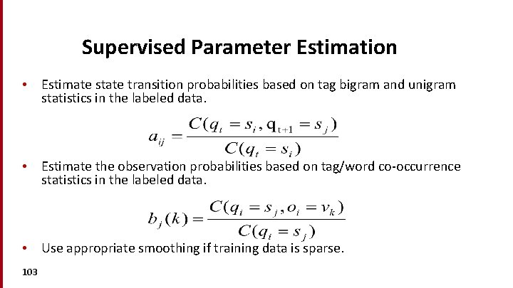
Supervised Parameter Estimation • Estimate state transition probabilities based on tag bigram and unigram statistics in the labeled data. • Estimate the observation probabilities based on tag/word co-occurrence statistics in the labeled data. • Use appropriate smoothing if training data is sparse. 103

Evaluating Taggers Train on training set of labeled sequences. Possibly tune parameters based on performance on a development set. Measure accuracy on a disjoint test set. Generally measure tagging accuracy, i. e. the percentage of tokens tagged correctly. • Accuracy of most modern POS taggers, including HMMs is 96− 97% (for Penn tagset trained on about 800 K words). Most freq. baseline: ~92. 4% • • • Generally matching human agreement level. 104