Wireless Sensor Networks Scaling and Deployment in Industrial

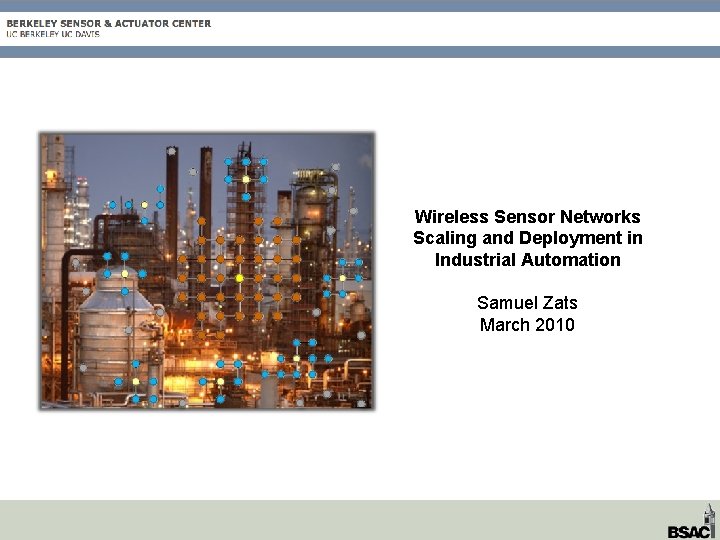
Wireless Sensor Networks Scaling and Deployment in Industrial Automation Samuel Zats March 2010

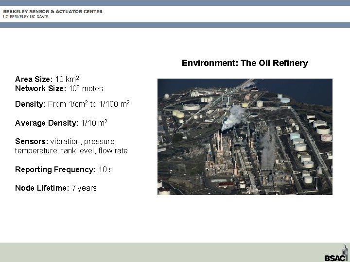
Environment: The Oil Refinery Area Size: 10 km 2 Network Size: 106 motes Density: From 1/cm 2 to 1/100 m 2 Average Density: 1/10 m 2 Sensors: vibration, pressure, temperature, tank level, flow rate Reporting Frequency: 10 s Node Lifetime: 7 years

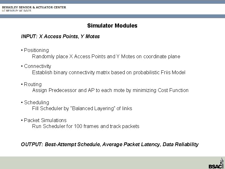
Simulator Modules INPUT: X Access Points, Y Motes • Positioning Randomly place X Access Points and Y Motes on coordinate plane • Connectivity Establish binary connectivity matrix based on probabilistic Friis Model • Routing Assign Predecessor and AP to each mote by minimizing Cost Function • Scheduling Fill Scheduler by “Balanced Layering” of links • Packet Simulations Run Scheduler for 100 frames and track packets OUTPUT: Best-Attempt Schedule, Average Packet Latency, Data Reliability

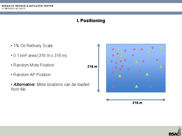
I. Positioning • 1% Oil Refinery Scale • 0. 1 km 2 area (316 m x 316 m) • Random Mote Position 316 m • Random AP Position • Alternative: Mote locations can be loaded from file. 316 m

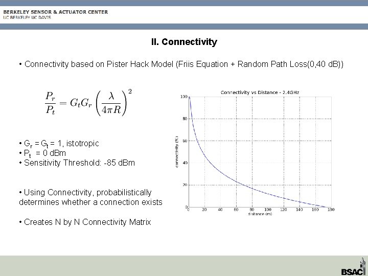
II. Connectivity • Connectivity based on Pister Hack Model (Friis Equation + Random Path Loss(0, 40 d. B)) • Gr = Gt = 1, istotropic • Pt = 0 d. Bm • Sensitivity Threshold: -85 d. Bm • Using Connectivity, probabilistically determines whether a connection exists • Creates N by N Connectivity Matrix

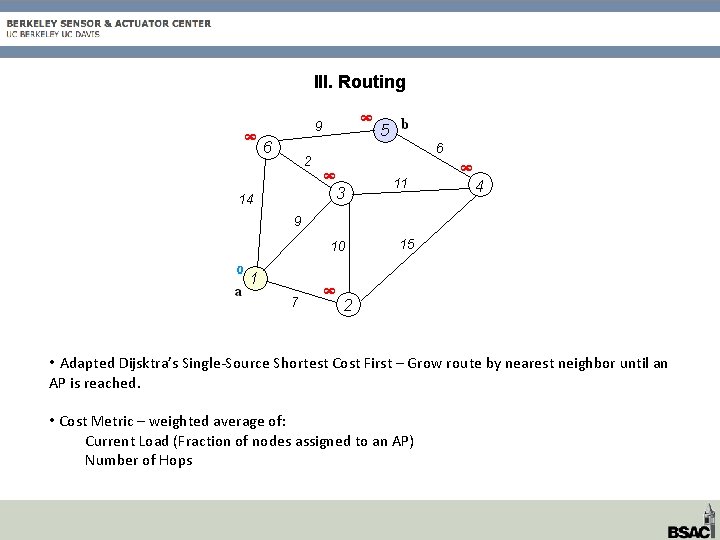
III. Routing • Adapted Dijsktra’s Single-Source Shortest Cost First – Grow route by nearest neighbor until an AP is reached. • Cost Metric – weighted average of: Current Load (Fraction of nodes assigned to an AP) Number of Hops

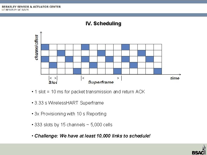
IV. Scheduling • 1 slot = 10 ms for packet transmission and return ACK • 3. 33 s Wireless. HART Superframe • 3 x Provisioning with 10 s Reporting • 333 slots by 15 channels ~ 5, 000 cells • Challenge: We have at least 10, 000 links to schedule!

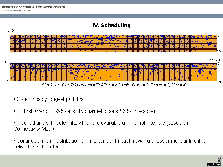
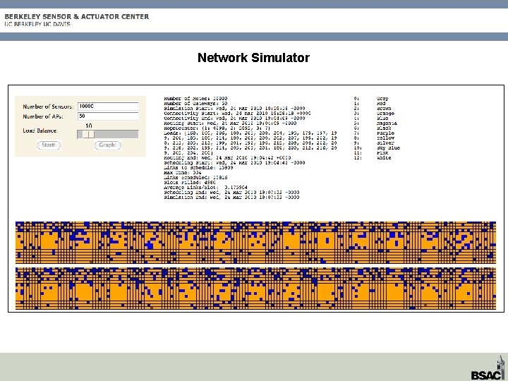
IV. Scheduling t=0 s 0 0 15 15 t = 333 0 0 15 Simulation of 10, 000 nodes with 50 APs (Link Counts: Brown = 2, Orange = 3, Blue = 4) • Order links by longest-path first • Fill first layer of 4, 995 cells (15 channel offsets * 333 time slots) • Proceed and schedule links which are available and do not interfere (based on Connectivity Matrix) • Continue uniform distribution of links per cell through row-major assignment until entire network is scheduled. 15

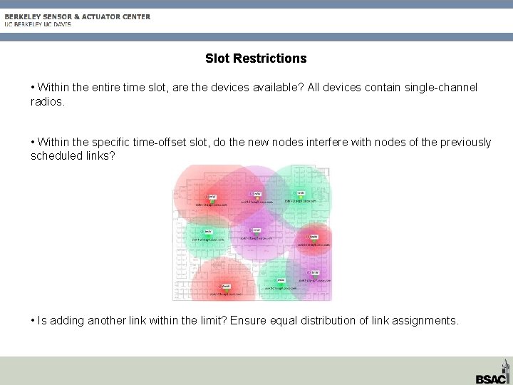
Slot Restrictions • Within the entire time slot, are the devices available? All devices contain single-channel radios. • Within the specific time-offset slot, do the new nodes interfere with nodes of the previously scheduled links? • Is adding another link within the limit? Ensure equal distribution of link assignments.

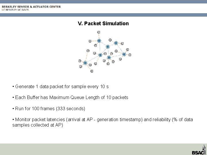
V. Packet Simulation • Generate 1 data packet for sample every 10 s • Each Buffer has Maximum Queue Length of 10 packets • Run for 100 frames (333 seconds) • Monitor packet latencies (arrival at AP - generation timestamp) and reliability (% of data samples collected at AP)

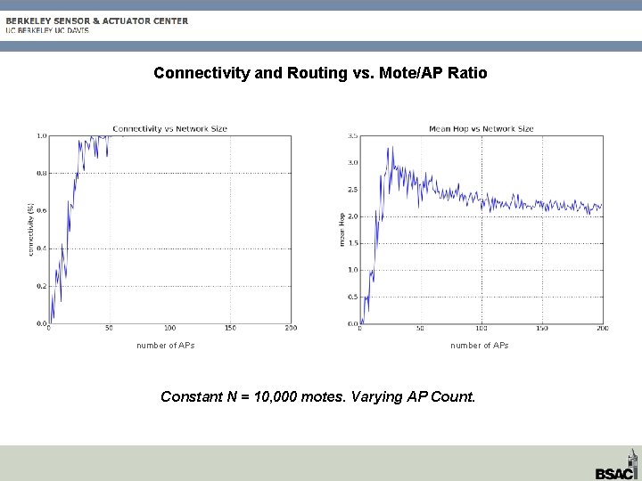
Connectivity and Routing vs. Mote/AP Ratio number of APs Constant N = 10, 000 motes. Varying AP Count.

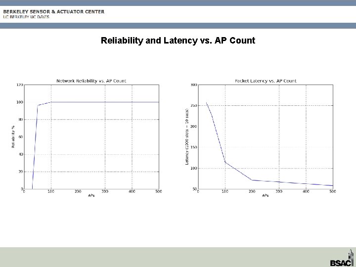
Reliability and Latency vs. AP Count

Network Simulator

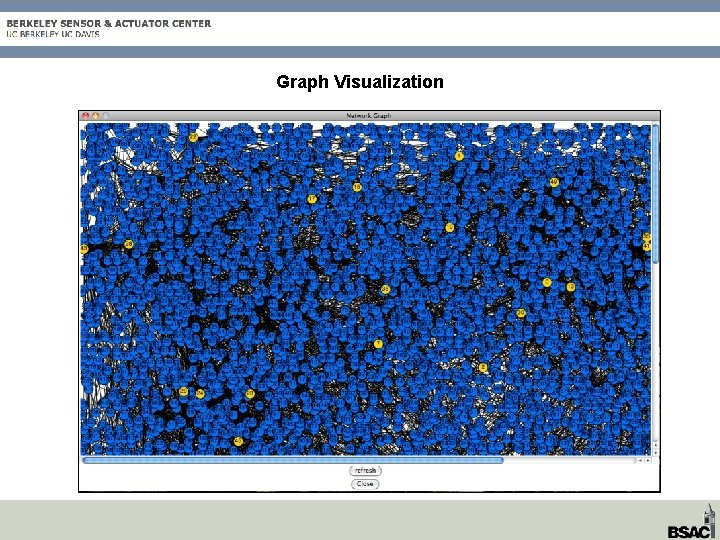
Graph Visualization

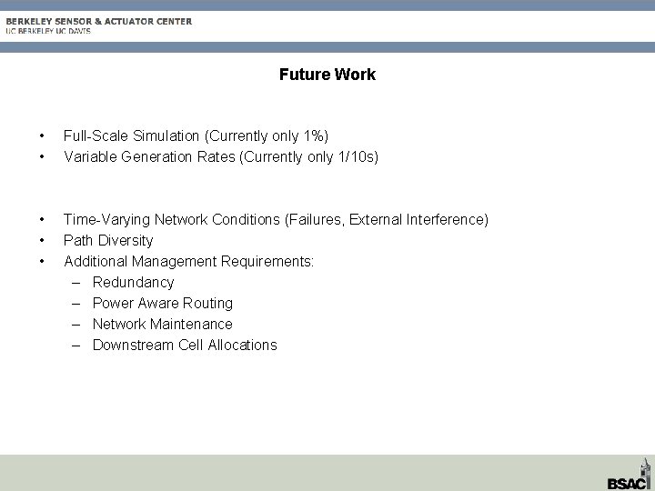
Future Work • • Full-Scale Simulation (Currently only 1%) Variable Generation Rates (Currently only 1/10 s) • • • Time-Varying Network Conditions (Failures, External Interference) Path Diversity Additional Management Requirements: – Redundancy – Power Aware Routing – Network Maintenance – Downstream Cell Allocations