Wireless Communications with GNU SDR Writing a signal

Wireless Communications with GNU SDR

Writing a signal processing block • • http: //www. nd. edu/~jnl/sdr/docs/tutorials/10. html As mentioned earlier, the signal processing is carried out by the signal processing blocks. The signal processing blocks are written in C++. Each block has input ports and output ports. A block is fed with input data and will spit output data. Multiple blocks are connected by the flow graph. Each block runs *in parallel* supported by threads. So keep in mind that you are writing a parallel program! There is a central scheduler which sets up buffers between the blocks and determines how much data each block should consume. Each block should also tell the scheduler how much data it has produced. It is the central scheduler’s job to keep the flow running without stalling. But you need to tell the scheduler the correct information.

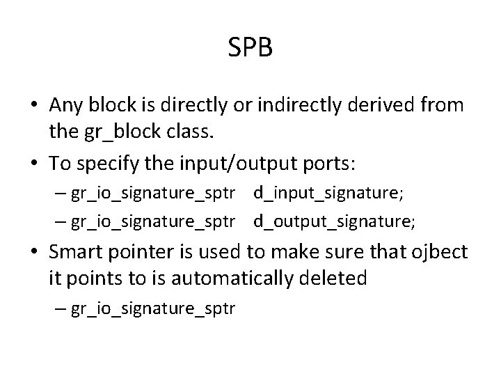
SPB • Any block is directly or indirectly derived from the gr_block class. • To specify the input/output ports: – gr_io_signature_sptr d_input_signature; – gr_io_signature_sptr d_output_signature; • Smart pointer is used to make sure that ojbect it points to is automatically deleted – gr_io_signature_sptr

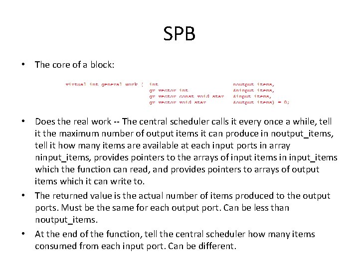
SPB • The core of a block: • Does the real work -- The central scheduler calls it every once a while, tell it the maximum number of output items it can produce in noutput_items, tell it how many items are available at each input ports in array ninput_items, provides pointers to the arrays of input items in input_items which the function can read, and provides pointers to arrays of output items which it can write to. • The returned value is the actual number of items produced to the output ports. Must be the same for each output port. Can be less than noutput_items. • At the end of the function, tell the central scheduler how many items consumed from each input port. Can be different.

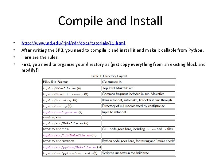
Compile and Install • • http: //www. nd. edu/~jnl/sdr/docs/tutorials/11. html After writing the SPB, you need to compile it and install it and make it callable from Python. Here are the rules. First, you need to organize your directory as (just copy everything from an existing block and modify!)

SPB • Then, you need to write a. i file to tell SWIG, the Simplified Wrapper and Interface Generator to generate the interface callable by Python. • The. i file is very small and normally you don’t have to do a lot with it except change the class names to the one you are currently using (the details in the online tutorial. ) • Then you need to modify Makefile. am, also just to update some names (the details in the online tutorial) • Then you need to modify configure. ac at the top directory, only two lines (the details in the online tutorial)

SPB • Then, run these commands. If your code is right everything should be fine.

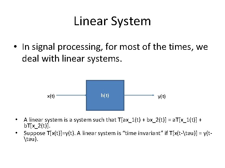
Linear System • In signal processing, for most of the times, we deal with linear systems. x(t) h(t) y(t) • A linear system is a system such that T[ax_1(t) + bx_2(t)] = a. T[x_1(t)] + b. T[x_2(t)]. • Suppose T[x(t)]=y(t). A linear system is “time invariant” if T[x(t-tau)] = y(ttau).

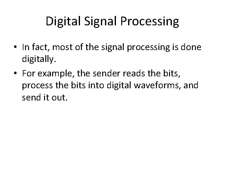
Digital Signal Processing • In fact, most of the signal processing is done digitally. • For example, the sender reads the bits, process the bits into digital waveforms, and send it out.

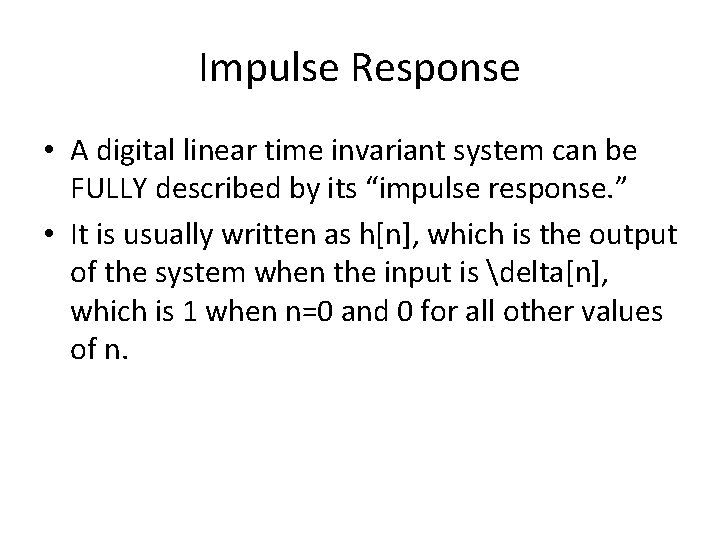
Impulse Response • A digital linear time invariant system can be FULLY described by its “impulse response. ” • It is usually written as h[n], which is the output of the system when the input is delta[n], which is 1 when n=0 and 0 for all other values of n.

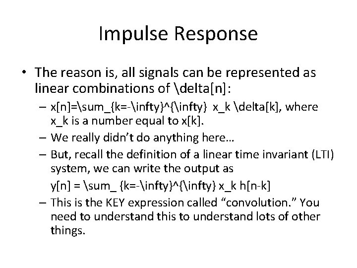
Impulse Response • The reason is, all signals can be represented as linear combinations of delta[n]: – x[n]=sum_{k=-infty}^{infty} x_k delta[k], where x_k is a number equal to x[k]. – We really didn’t do anything here… – But, recall the definition of a linear time invariant (LTI) system, we can write the output as y[n] = sum_ {k=-infty}^{infty} x_k h[n-k] – This is the KEY expression called “convolution. ” You need to understand this to understand lots of other things.

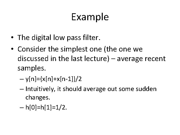
Example • The digital low pass filter. • Consider the simplest one (the one we discussed in the last lecture) – average recent samples. – y[n]={x[n]+x[n-1]}/2 – Intuitively, it should average out some sudden changes. – h[0]=h[1]=1/2.

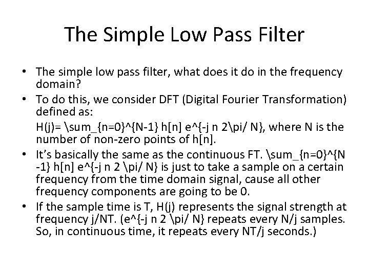
The Simple Low Pass Filter • The simple low pass filter, what does it do in the frequency domain? • To do this, we consider DFT (Digital Fourier Transformation) defined as: H(j)= sum_{n=0}^{N-1} h[n] e^{-j n 2pi/ N}, where N is the number of non-zero points of h[n]. • It’s basically the same as the continuous FT. sum_{n=0}^{N -1} h[n] e^{-j n 2 pi/ N} is just to take a sample on a certain frequency from the time domain signal, cause all other frequency components are going to be 0. • If the sample time is T, H(j) represents the signal strength at frequency j/NT. (e^{-j n 2 pi/ N} repeats every N/j samples. So, in continuous time, it repeats every NT/j seconds. )

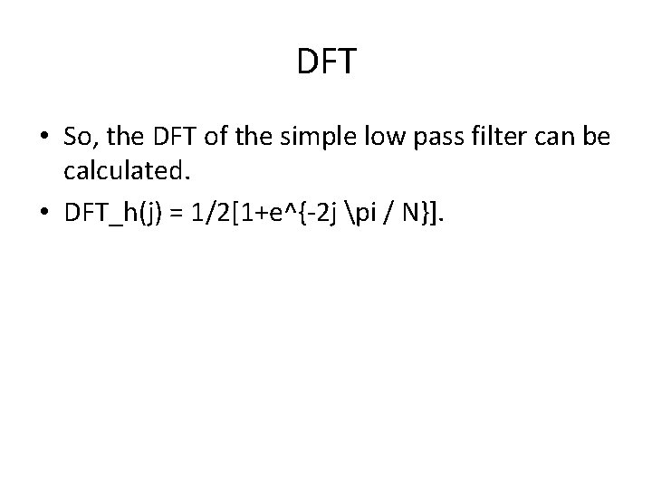
DFT • So, the DFT of the simple low pass filter can be calculated. • DFT_h(j) = 1/2[1+e^{-2 j pi / N}].

Convolution and Frequency

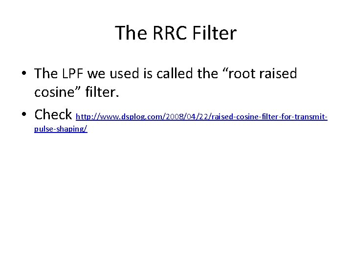
The RRC Filter • The LPF we used is called the “root raised cosine” filter. • Check http: //www. dsplog. com/2008/04/22/raised-cosine-filter-for-transmitpulse-shaping/

Why use RC • The problem is that the baseband waveform is generated but you have to take samples at the receiver side to determine the bits. • If using some arbitrary LPF, the signal shape is arbitrary and the samples you take for y[n] will have interferences from y[n-1], y[n-2], …, y[n+1], y[n+2]… • So you want to use LPF such that all other non-relevant samples have 0 influence on the current sample. • The Raised Cosine Filter satisfies this constraint • Root means that the sender and receiver will each do half of it.

Carrier Phase Tracking

Sample Time