Windowing Purpose process pieces of a signal and

Windowing • Purpose: process pieces of a signal and minimize impact to the frequency domain • Using a window – First Create the window: Use the window formula to calculate an array of window values – Next apply the window: multiply these values by each time domain amplitude in a frame • Window Length: The number of signal values in a frame is the window length

Example: Hamming Window • Create Window double[] window = new double[window. Size]; double c = 2*Math. PI / (window. Size - 1); for (int h=0; h<window. Size; h++) window[h] = 0. 54 - 0. 46*Math. cos(c*h); • Apply window for(int i=0; i<window. length; i++) frame[i]=frame[i]*window[i]; • Note: Time domain multiplication is frequency domain convolution. Therefore, windows act as a frequency domain filter.

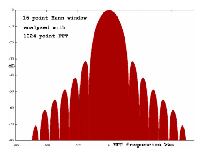
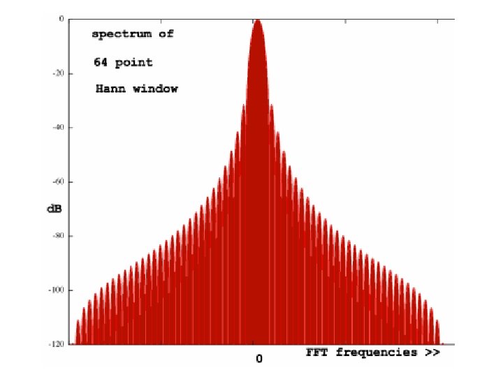
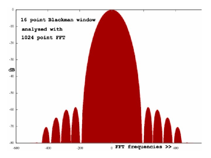
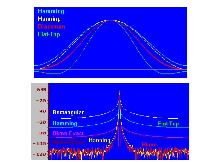
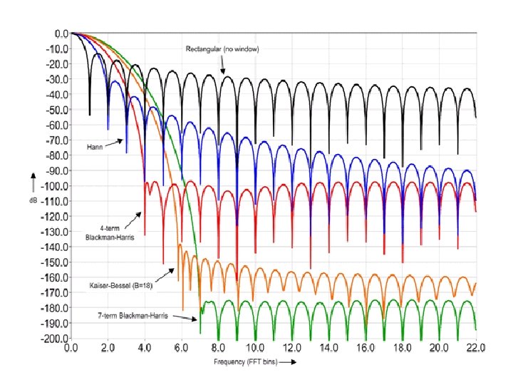
Windowing Frequency Response • Main Lobe: Narrow implies better frequency resolution. As the window length grows, the main lobe width narrows (less initial spectral leakage). • Side lobe: Higher for abrupt time domain window transitions from 1 to 0. • Roll-off rate: Slower for abrupt window discontinuities. Spectral Leakage: Side Lobe Roll-off Rate Some of the spectral energy leaks into other frequency bins, which blur frequency distinctions. Note: some windows act as a amplifier of total energy Main Lobe

Rectangular Frequency Response • Fourier transform of r(x): R(f) = ∫∞, ∞r(x) e-2πxfidt • r(x) is zero outside ±T/2: R(f) = ∫-T/2, T/2 1. e-2πftidt • Chain Rule: The integral of e-2πfti is e-2πfti /(-2πfi) R(f) = e-2πfti /(-2πfti)|T/2, -T/2 = e-2πf. T/2 i/(-2πfi) - e-2πf(-T/2)i/(-2πfi) • By Eulers formula: R(f) = (eπf. Ti - e-πf. Ti)/(2πfi) = sin(πf. T)/(πf. T)

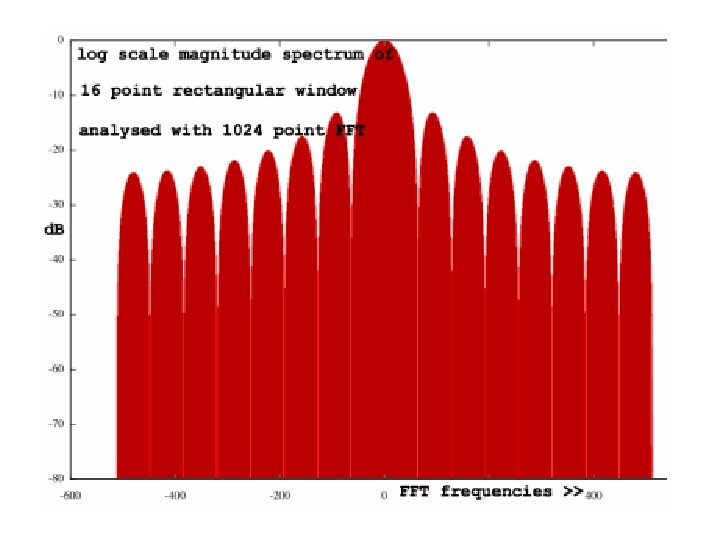
Rectangular Window • Main lobe width: 4π/M, Side lobe width: 2 π /M • Minimal leakage, but directed to places that hurt analysis • Poor roll off and high initial lobe

Convoluting Rectangular Window with a particular frequency Note: Windows with more points narrow the central lobe

Triangular (Bartlett Window)

Compare: Hamming to Hanning Hamming Hanning: Faster roll of; Hamming: lower first lobe

Evaluation: Non-Rectangular • Greater total leakage, but redistributed to places where analysis is not affected. • If little energy spills outside the main lobe, it is harder to resolve frequencies that are near to each other. • Fast roll-off implies wide initial lobe and higher side lobe; worse at detecting weak sinusoids amidst noise. • Moderate roll-off, implies narrower initial lobe and lower side lobe. • Tradeoff: Resolving comparable strength signals with similar frequencies (moderate) and resolving disparate strength signals with dissimilar frequencies (fast roll-off).

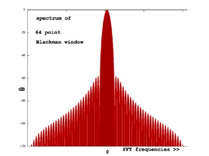
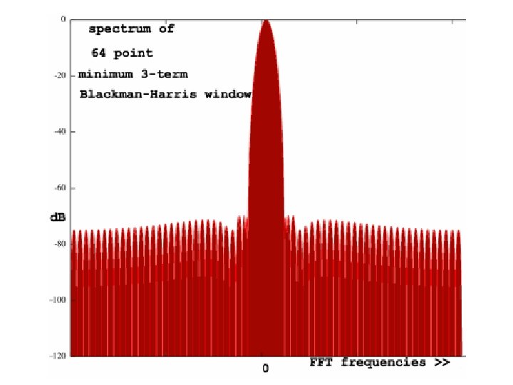
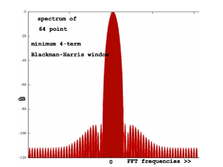
Windowing Formulae • • • Hanning: w[n] = 0. 5 -0. 5 cos(2πn/(N-1)) Hamming: w[n] = 0. 54 – 0. 45 cos(2πn/(N-1)) Bartlett: w[n] = 2/(N-1)/2 - |(n–(N-1)/2|) Triangle: w[n] = 2/N. (N/2 - |(n–(N-1)/2|) Blackman: w[n] = a 0 – a 1 cos(2πn/(N-1)) – a 2 cos(4πn/(N-1)) where: a 0 = (1 -α)/2 ; a 1 = ½ ; a 2 = α /2; α =0. 16 • Blackman-Harris: w[n] = a 0–a 1 cos(2πn/(N-1))–a 2 cos(4πn/(N-1)) - a 3 cos(6πn/(N-1)) where: a 0=0. 35875; a 1=0. 48829; a 2=0. 14128; a 3=0. 01168 Note: Small formula changes can cause large frequency response differences

Moving Average Filters • Both filters can be used to smooth a signal and reduce noise • It curves sharp angles in the time domain. • It overreacts to outlier samples • Slow roll-off destroys ability to separate frequency bands • Horrible stop band attenuation • Evaluation – An exceptionally good smoothing filter – An exceptionally bad low-pass filter

Moving Average Filter • FIR version: • Yn = 1/M ∑i=0, M-1 xn-I • Slower than the IIR version • IIR version: • yn = yn-1 + (xn – xn-M)/M • Propagates rounding errors • Example: {1, 2, 3, 4, 5, 4, 3, 2, 1, 2, 3, 4, 5}; M = 4 – Starting filtered values: {¼ , ¾, 1 ½, 2 ½, … } – Next value using the FIR version: Y 4 = ¼(5+4+3+2) = 3 ½ – Next value using the IIR version: y 4 = 2 ½ + (5 – 1)/4 = 3 ½ – Not appropriate for speech because: – Blurs transitions between voiced/unvoiced sounds – Negatively impacts the frequency domain

Median Filter

Median Filter • Median definition: – The middle value of an ordered list – If there is no middle value, average the two middle values • Median filter: Yn = medianm=0, M-1 {xn-m} • Advantages – Good edge preserving properties – Preserves sharp discontinuities of significant length – Eliminates outliers • Applications – The most effective algorithm to removes sudden impulse noise – Remove outliers in estimates of a pitch contour • Implementation: Requires maintaining a running sorted list

Characteristics: Median Filter • Linearity tests ØFails: an * Mn + bn * Mn ≠ (an + bn) * Mn ØSucceeds: α (an)*Mn = (α an)*Mn ØSucceeds: An * Mn = bn, then An+k * Mn+k = bn+k • Every output will match an input (if the filter length is odd) • Frequency response • There is not a mathematic formula • Must be determined experimentally

Double Smoothing 1. 2. 3. 4. Apply a median filter (ex: five point) and then a Apply a linear filter (Ex: Hanning with values 0, ¼ , ½ , ¼, 0) Recursively apply steps 1 and 2 to the filtered signal Add the result of the recursive application back Single Smoothing Double Smoothing

Compare Median to Moving Average Filter