Why you should know about experimental crosses Why

Why you should know about experimental crosses

Why you should know about experimental crosses To save you from embarrassment

Why you should know about experimental crosses To save you from embarrassment To help you understand analyse human genetic data

Why you should know about experimental crosses To save you from embarrassment To help you understand analyse human genetic data It’s interesting

Experimental crosses

Experimental crosses Inbred strain crosses Recombinant inbreds Alternatives

Inbred Strain Cross

Backcross

F 2 cross Generation F 0 F 1 F 2

Data conventions AA = A BB = B AB = H Missing data = -

Data conventions Genotype file

Data conventions Genotype file Phenotype file

Data conventions Genotype file Phenotype file Map file

Map file Use the latest mouse build and convert physical to genetic distance: 1 Mb = 1. 6 c. M Use our genetic map: http: //gscan. well. ox. ac. uk/

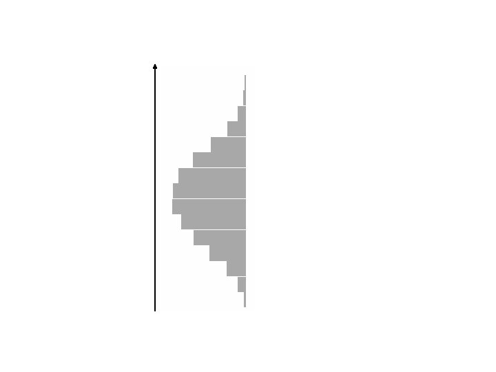
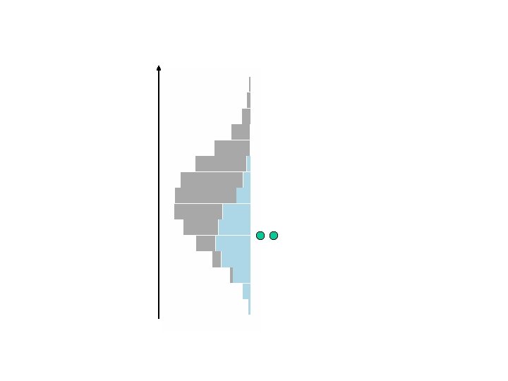
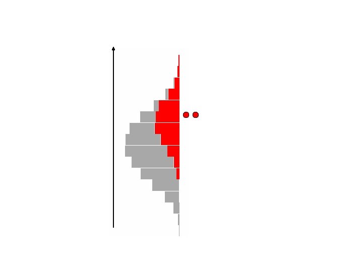
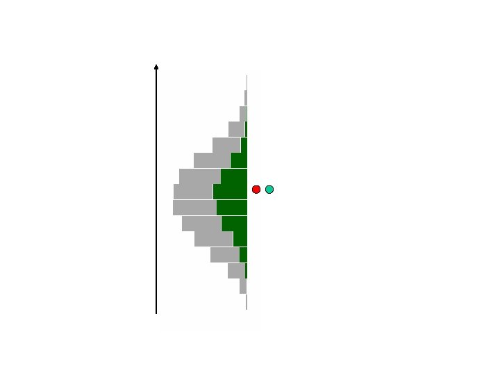
Analysis If you can’t see the effect it probably isn’t there

1400 1200 Phenotype 1000 800 600 400 200 0 0. 5 AA AB BB

Red = Hom Blue = Het Backcross genotypes

Statistical analysis

Linear models Also known as ANOVA ANCOVA regression multiple regression linear regression

QTL snp

+1 0 -1 QTL snp

+1 0 -1 QTL snp

+1 0 -1 QTL snp

+1 0 -1 QTL snp

qq q. Q QQ

QTL snp +1 0 0 1 -1 0

QTL snp +1 0 0 1 -1 0

100 90 90 80 qq q. Q QQ 10 0

100 90 80 qq q. Q QQ 90 10 0 90 10 10

Hypothesis testing H 0 : H 1 :

Hypothesis testing H 0 : y ~1 H 1 : y~1+x

Hypothesis testing H 0 : y~1 H 1 : y~1+x H 1 vs H 0 : Does x explain a significant amount of the variation?

Hypothesis testing H 0 : y~1 H 1 : y~1+x H 1 vs H 0 : Does x explain a significant amount of the variation? LOD score likelihood ratio

Hypothesis testing H 0 : y~1 H 1 : y~1+x H 1 vs H 0 : Does x explain a significant amount of the variation? LOD score likelihood ratio Chi Square test p-value log. P

Hypothesis testing H 0 : y~1 H 1 : y~1+x H 1 vs H 0 : Does x explain a significant amount of the variation? LOD score likelihood ratio linear models only SS explained / SS unexplained Chi Square test F-test (or t-test) p-value log. P

Hypothesis testing H 0 : y~1+x H 1 : y ~ 1 + x 2 H 1 vs H 0 : Does x 2 explain a significant extra amount of the variation?

PRACTICAL: hypothesis test for identifying QTLs To start: 1. Copy the folder facultyvaldarAnimal. Models. Practical to your own directory. 2. Start R 3. File -> Change Dir… and change directory to your Animal. Models. Practical directory 4. Open Firefox, then File -> Open File, and open “f 2 cross_and_thresholds. R” in the Animal. Models. Practical directory H 0 : phenotype ~ 1 H 1 : phenotype ~ a H 2 : phenotype ~ a + d Test: H 1 vs H 0 H 2 vs H 1 H 2 vs H 0

PRACTICAL: Chromosome scan of F 2 cross

Two problems in QTL analysis Missing genotype problem Model selection problem

Missing genotype problem

Solutions to the missing genotype problem Maximum likelihood interval mapping Haley-Knott regression Multiple imputation

Interval mapping

Interval mapping qq genotype 10 q. Q genotype 20

Interval mapping qq genotype 10 q. Q genotype 20

Interval mapping qq genotype 10 q. Q genotype 20 Which is the true situation? qq q. Q

Interval mapping qq genotype 10 q. Q genotype 20 Which is the true situation? qq Fit both situations and then weight them 0. 5 “mixture” model q. Q 0. 5 ML interval mapping

Interval mapping qq genotype 10 q. Q genotype 20 Which is the true situation? qq Fit both situations and then weight them 0. 5 “mixture” model q. Q 0. 5 ML interval mapping Fit the “average” situation (which is technically false, but quicker) Haley-Knott regression

Imputation

Imputation

Key references Maximum likelihood methods Linear regression Imputation

r/qtl http: //www. rqtl. org/ Broman, Sen & Churchill

Is interval mapping necessary?

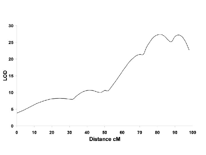
QTL log. P score

QTL

QTL log. P score

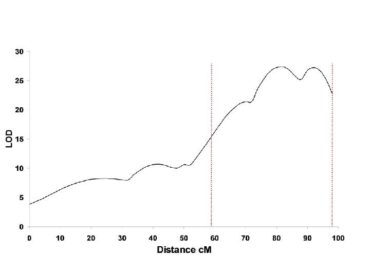
Significance Thresholds

Significance Thresholds Lander, E. Kruglyak, L. Genetic dissection of complex traits: guidelines for interpreting and reporting linkage results Nature Genetics. 11, 2417, 1995

Thresholds Permutation test SUBJECT. NAME Sex Phenotype m 1 m 2 m 3 m 4 F 2$798 F -0. 738004 -1 1 1 -1 F 2$364 F 0. 413330 0 0 F 2$367 F 1. 417480 -1 1 1 -1 F 2$287 F 0. 811208 1 -1 -1 1 F 2$205 M 1. 198270 0 0

Thresholds Permutation test SUBJECT. NAME Sex Phenotype m 1 m 2 m 3 m 4 F 2$798 F -0. 738004 -1 1 1 -1 F 2$364 F 0. 413330 0 0 F 2$367 F 1. 417480 -1 1 1 -1 F 2$287 F 0. 811208 1 -1 -1 1 F 2$205 M 1. 198270 0 0 shuffle SUBJECT. NAME Sex Phenotype m 1 m 2 m 3 m 4 F 2$798 F 0. 413330 -1 1 1 -1 F 2$364 F 1. 417480 0 0 F 2$367 F 1. 198270 -1 1 1 -1 F 2$287 F -0. 738004 1 -1 -1 1 F 2$205 M 0. 811208 0 0

Permutation tests to establish thresholds Empirical threshold values for quantitative trait mapping GA Churchill and RW Doerge Genetics, 138, 963 -971 1994 An empirical method is described, based on the concept of a permutation test, for estimating threshold values that are tailored to the experimental data at hand.

PRACTICAL: significance thresholds by permutation

Two problems in QTL analysis Missing genotype problem Model selection problem

The model problem How QTL genotypes combine to produce the phenotype

The model problem Linked QTL corrupt the position estimates Unlinked QTL decreases the power of QTL detection

Composite interval mapping ZB Zeng Precision mapping of quantitative trait loci Genetics, Vol 136, 1457 -1468, 1994 http: //statgen. ncsu. edu/qtlcart/cartographer. html

Composite interval mapping Q M 1 Q M 2 Q

Composite interval mapping Q M-1 M 1 Q M 2 M 3 Q

Model selection Inclusion of covariates: gender, environment and other things too many too enumerate here

Inclusion of covariates H 0 : phenotype ~ covariates H 1 : phenotype ~ covariates + Locus. X

Inclusion of covariates H 0 : phenotype ~ covariates H 1 : phenotype ~ covariates + Locus. X H 1 vs H 0 : how much extra does Locus. X explain?

Inclusion of covariates H 0 : phenotype ~ covariates H 1 : phenotype ~ covariates + Locus. X H 1 vs H 0 : how much extra does Locus. X explain? H 0 : startle ~ Sex + Body. Weight + Test. Chamber + Age H 1 : startle ~ Sex + Body. Weight + Test. Chamber + Age + Locus 432

PRACTICAL: Inclusion of gender effects in a genome scan To start: In Firefox, then File -> Open File, and open “gxe. R”

Experimental crosses Inbred strain crosses Recombinant inbreds Alternatives

Recombinant Inbreds F 0 Parental Generation F 1 Generation F 2 Generation Interbreeding for approximately 20 generations to produce recombinant inbreds

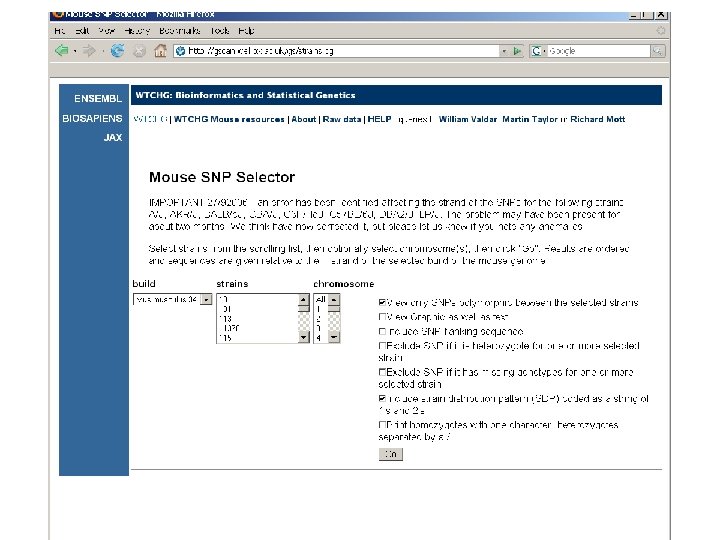
RI strain genotypes http: //www. well. ox. ac. uk/mouse/INBREDS SNP SELECTOR http: //gscan. well. ox. ac. uk/gs/strains. cgi

RI strain phenotypes

RI analysis

Power of RIs Effect size of a QTL that can be detected with RI strain sets, at P= 0. 00013

Experimental crosses Inbred strain crosses Recombinant inbreds Alternatives

Why do we need alternatives? Classical strategies don’t find genes because of poor resolution

One locus may contain many QTL

New approaches Chromosome substitution strains

New approaches Chromosome substitution strains Collaborative cross

New approaches Chromosome substitution strains Collaborative cross In silico mapping

Resources R http: //www. r-project. org/ R help http: //news. gmane. org/gmane. comp. lang. r. general R/qtl http: //www. rqtl. org Composite interval mapping (QTL Cartographer) Markers http: //statgen. ncsu. edu/qtlcart/index. php http: //www. well. ox. ac. uk/mouse/inbreds Gscan (HAPPY and associated analyses) http: //gscan. well. ox. ac. uk General reading Lynch & Walsh (1998) Genetics and analysis of quantitative traits (Sinauer). Dalgaard (2002) Introductory statistics with R (Springer-Verlag).

END SECTION


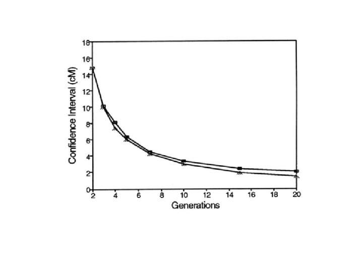
New approaches Advanced intercross lines Genetically heterogeneous stocks

F 2 Intercross x F 1 Avg. Distance Between Recombinations F 2 intercross ~30 c. M F 2
 F 0 F 1 F 2 F 3 F 4")
Advanced intercross lines (AILs) F 0 F 1 F 2 F 3 F 4
 significance threshold 0")
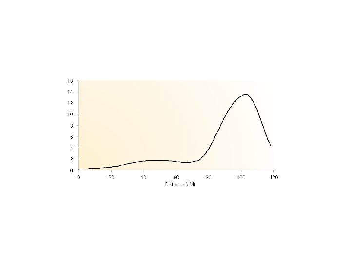
Chromosome scan for F 12 QTL goodness of fit (log. P) significance threshold 0 Typical chromosome position along whole chromosome (Mb) 100 c. M

PRACTICAL: AILs

Genetically Heterogeneous Mice

F 2 Intercross x F 1 Avg. Distance Between Recombinations F 2 intercross ~30 c. M F 2

Heterogeneous Stock F 2 Intercross x Pseudo-random mating for 50 generations F 1 Avg. Distance Between Recombinations: HS ~2 c. M F 2 intercross ~30 c. M F 2

Heterogeneous Stock F 2 Intercross x Pseudo-random mating for 50 generations F 1 Avg. Distance Between Recombinations: HS ~2 c. M F 2 intercross ~30 c. M F 2

Genome scans with single marker association

High resolution mapping

Relation Between Marker and Genetic Effect QTL Marker 1 Observable effect

Relation Between Marker and Genetic Effect Marker 2 QTL Marker 1 Observable effect

Relation Between Marker and Genetic Effect Marker 2 No effect observable QTL Marker 1 Observable effect
 calculates the probability that an allele descends from a founder using")
Multipoint method (HAPPY) calculates the probability that an allele descends from a founder using multiple markers Observed chromosome structure Hidden Chromosome Structure

M 1 m 1 Q q M 2 m 2 M 1 recombination ? m 2

Haplotype reconstruction using HAPPY A typical chromosome from an HS mouse m 183 m 184 m 185 allele

Haplotype reconstruction using HAPPY A typical chromosome from an HS mouse m 183 m 184 m 185 another plausible path actual path allele

Haplotype reconstruction using HAPPY A typical chromosome from an HS mouse m 183 m 184 m 185 another plausible path actual path allele

Haplotype reconstruction using HAPPY A typical chromosome from an HS mouse marker interval m 183 m 184 m 185 average over all paths allele

Haplotype reconstruction using HAPPY chromosome genotypes haplotype proportions predicted by HAPPY

HAPPY model for additive effects

HAPPY model for additive effects Phenotype y is modeled as is effect of strain s
 model")
HAPPY effects models Additive model with covariate effects Full (ie, additive & dominance) model with covariate effects

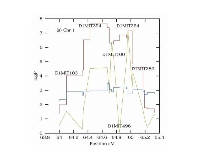
Genome scans with HAPPY

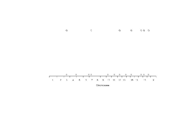
Many peaks mean red cell volume

Ghost peaks

family effects, cage effects, odd breeding …complex pattern of linkage disequilibrium


How to select peaks: a simulated example

How to select peaks: a simulated example Simulate 7 x 5% QTLs (ie, 35% genetic effect) + 20% shared environment effect + 45% noise = 100% variance

Simulated example: 1 D scan

Peaks from 1 D scan phenotype ~ covariates + ?

1 D scan: condition on 1 peak phenotype ~ covariates + peak 1 + ?

1 D scan: condition on 2 peaks phenotype ~ covariates + peak 1 + peak 2 + ?

1 D scan: condition on 3 peaks phenotype ~ covariates + peak 1 + peak 2 + peak 3 + ?

1 D scan: condition on 4 peaks phenotype ~ covariates + peak 1 + peak 2 + peak 3 + peak 4 + ?

1 D scan: condition on 5 peaks phenotype ~ covariates + peak 1 + peak 2 + peak 3 + peak 4 + peak 5 + ?

1 D scan: condition on 6 peaks phenotype ~ covariates + peak 1 + peak 2 + peak 3 + peak 4 + peak 5 + peak 6 + ?

1 D scan: condition on 7 peaks phenotype ~ covariates + peak 1 + peak 2 + peak 3 + peak 4 + peak 5 + peak 6 + peak 7 + ?

1 D scan: condition on 8 peaks phenotype ~ covariates + peak 1 + peak 2 + peak 3 + peak 4 + peak 5 + peak 6 + peak 7 + peak 8 + ?

1 D scan: condition on 9 peaks phenotype ~ covariates + peak 1 + peak 2 + peak 3 + peak 4 + peak 5 + peak 6 + peak 7 + peak 8 + peak 9 +?

1 D scan: condition on 10 peaks phenotype ~ covariates + peak 1 + peak 2 + peak 3 + peak 4 + peak 5 + peak 6 + peak 7 + peak 8 + peak 9 + peak 10 + ?

1 D scan: condition on 11 peaks phenotype ~ covariates + peak 1 + peak 2 + peak 3 + peak 4 + peak 5 + peak 6 + peak 7 + peak 8 + peak 9 + peak 10 + peak 11 + ?

Peaks chosen by forward selection

Bootstrap sampling 1 2 3 10 subjects 4 5 6 7 8 9 10

Bootstrap sampling sample with replacement 10 subjects 1 1 2 2 3 2 4 3 5 5 6 5 7 6 8 7 9 7 10 9 bootstrap sample from 10 subjects

Forward selection on a bootstrap sample

Forward selection on a bootstrap sample

Forward selection on a bootstrap sample

Bootstrap evidence mounts up…
")
In 1000 bootstraps… Bootstrap Posterior Probability (BPP)

Model averaging by bootstrap aggregation Choosing only one model: very data-dependent, arbitrary can’t get all the true QTLs in one model Bootstrap aggregation averages over models true QTLs get included more often than false ones References: Broman & Speed (2002) Hackett et al (2001)

PRACTICAL: http: //gscan. well. ox. ac. uk

ADDITIONAL SLIDES FROM HERE

An individual’s phenotype follows a mixture of normal distributions

Paternal chromosome Maternal chromosome m

m Chromosome 1 Chromosome 2 Strains A B C D E F

Markers m Strains A B C D E F

Markers m Strains A B C D E F

Markers m 0. 5 c. M

Markers m 0. 5 c. M 1 c. M

Markers 0. 5 c. M 1 c. M m
: implemented in HAPPY http: //www. well. ox.")
Analysis Probabilistic Ancestral Haplotype Reconstruction (descent mapping): implemented in HAPPY http: //www. well. ox. ac. uk/~rmott/happy. html

M 1 m 1 Q q M 2 m 2 M 1 recombination ? m 2

m 1 M 1 M 1 m 1 Q q q Q q M 2 m 2

m 1 M 1 M 1 m 1 Q q q Q q M 2 m 2 M 1 m 1 M 1 Q q Q m 2 M 2 m 2

M 1 m 1 M 1 Q q q m 2 m 2 m 1 M 1 Q q Q M 2 m 2 m 1 Q q M 2 m 2

M 1 m 1 ? ? m 2 c. M distances determine probabilities

M 1 Eg, m 1 ? ? m 2 c. M distances determine probabilities

Interval mapping M 1 M 2 m 1 m 2 LOD score M 1 m 1 M 2 m 2

Interval mapping M 1 m 1 Q q M 2 m 2 LOD score M 1 m 1 M 2 m 2

Interval mapping M 1 m 1 Q q M 2 m 2 LOD score M 1 m 1 M 2 m 2

Interval mapping M 1 m 1 Q q M 2 m 2 LOD score M 1 m 1 M 2 m 2
- Slides: 172