Why Probability Originally devised for gambling by Pascal

Why Probability? • Originally devised for gambling by Pascal and Laplace over 200 years ago. • Current applications of probability include genetics study (e. g. , to understand inheritance of traits) and computer science (e. g. , to determine average-case complexity of algorithms).

Definitions • Experiments: a procedure that yields one of a given set of possible outcomes. • Sample space of an experiment: the set of possible outcomes. • Event: a subset of the sample space whose outcome is of our interest. • Probability of an event, p(E) = |E|/|S|

Examples • Ex 1: What’s the probability of drawing a blue ball from an urn containing four blue balls and five red balls? [4/(4+5) = 4/9] • Ex 2: What’s the probability that when two dice are rolled, the sum of the numbers on the two dice is 7? – Number of possible outcomes, |S|, = 6*6 = 36 – Events where the sum of the numbers is 7 include (1, 6), (2, 5), (3, 4), (4, 3), (5, 2), (6, 1) |E| = 6 – The probability of such event, p(E), = |E|/|S| = 6/36 = 1/6

More examples • Ex 3: Find the probability that a hand of five cards in poker contains four cards of one kind? – Sample space, S, is number of possible ways to choose 5 cards out of 52 cards |S| = C(52, 5) – Event, E, to select four cards of one kind, includes first select 1 kind out of 13 kinds (C(13, 1)), then select 4 cards of this kind from the four in the deck of this kind (C(4, 4)), and finally select 1 last card out of the 48 cards left (C(48, 1)) – Probability, p(E) = |E|/|S| =

Complementary probability • Theorem 1: Let E be an event in a sample space S. The probability of the event , the complementary event of E, is given by • Ex: A sequence of ten bits is randomly generated. What’s the probability that at least one of these bits is 0? – E = event that at least one of ten bits is 0 = event that all bits are 1 s. – p(E) = 1 – p( ) = 1 – 1/210 = 1 – 1/1024 = 1023/1024

Probability of union of two events • Theorem 2: Let E 1 and E 2 be events in the sample space S. Then (by the inclusion-exclusion principle), p(E 1 E 2) = p(E 1) + p(E 2) – p(E 1 E 2)

Properties of probability values 1. 2. The probability of each outcome is a nonnegative real number no greater than 1. That is, 0 p(xi) 1 for i = 1, 2, …, n The sum of the probabilities of all possible outcomes should be 1. That is, Such a p is called a probability distribution Definition 2: The probability of the event E is the sum of the probabilities of the outcomes in E. That is,

Probability • The probability p = p(E) [0, 1] of an event E is a real number representing our degree of certainty that E will occur. – If p(E) = 1, then E is absolutely certain to occur, – If p(E) = 0, then E is absolutely certain not to occur, – If p(E) = ½, then we are completely uncertain about whether E will occur. – What about other cases?

An Example • Ex: What’s the probability that an odd number appears when we roll a die with equally likely outcomes? – probability of the event an odd number appears, E, = {1, 3, 5}. Each event has probability p(1) = p(3) = p(5) = 1/6 – Therefore, p(E) = p(1) + p(3) = p(5) = 3/6 = 1/2

Random Variables • A random variable V is a variable whose value is unknown, or that depends on the situation. – E. g. , the number of students in class today – the grades students receive in this class – Whether it will rain tonight (Boolean variable) • The proposition V=vi may be uncertain, and be assigned a probability.

Mutually Exclusive Events • Two events E 1, E 2 are called mutually exclusive if they are disjoint: E 1 E 2 = • Note that two mutually exclusive events cannot both occur in the same instance of a given experiment. • For mutually exclusive events, p(E 1 E 2) = p(E 1) + p(E 2).

Exhaustive Sets of Events • A set E = {E 1, E 2, …} of events in the sample space S is exhaustive if. • An exhaustive set of events that are all mutually exclusive with each other has the property that

Conditional Probability • Let E, F be events such that p(F)>0. • Then, the conditional probability of E given F, written p(E|F), is defined as p(E|F) = p(E F)/p(F). • This is the probability that E would turn out to be true, given just the information that F is true. • If E and F are independent, p(E|F) = p(E).

An Example • Ex 1: A bit string of length four is generated at random so that each of the 16 bit strings of length four is equally likely. What’s the probability that it contains at least two consecutive 0 s given that its first bit is 0? • Let E = event that a bit string of length four contains at least two consecutive 0 s, and • let F = event that the first bit of a bit string of length four is a 0. Then, p(E|F) = p(E F)/p(F) • E F = {0000, 0001, 0010, 0011, 0100} p(E F) = 5/24 = 5/16. Since half of the bit string of length four must begin with 0 (the other half begins with 1), p(F) = 8/16 = ½. Therefore, p(E|F) = (5/16)/(1/2) = 5/8

Independent Events • Two events E, F are independent if and only if p(E F) = p(E)·p(F). • Relates to product rule for number of ways of doing two independent tasks • Example: Flip a coin, and roll a die. p( quarter is heads die is 1 ) = p(quarter is heads) × p(die is 1)

Bernoulli Trials • Theorem 2: The probability of exactly k successes in n independent Bernoulli trials, with probability of success p and probability of failure q = 1 – p, is C(n, k) pk qn-k

An Example • Ex: What’s the probability that exactly four heads come up when a fair coin is flipped seven times, assuming that the flips are independent. • n = 7, k = 4, n – k = 7 – 4 = 3 • p = probability of success (getting head) = ½ • q=1–p=½ • Therefore, p(gets 4 heads out of 7 flips) = C(n, k) pk qn-k = C(7, 4) (1/2)4(1/2)3

Bayes’s Theorem • Allows one to compute the probability that a hypothesis H is correct, given data D: • Easy to prove from def’n of conditional prob. • Extremely useful in artificial intelligence apps: – Data mining, automated diagnosis, pattern recognition, statistical modeling, evaluating scientific hypotheses.

Expectation Values • For a random variable X(s) on the sample space S is equal to E(X) = ∑s S p(s)X(s) • The term “expected value” is widely used, but misleading since the expected value might be totally unexpected or impossible! • Ex 1: Let X be the number that comes up when a die is rolled. What’s the expected value of X? Random variable X takes the values 1, 2, 3, 4, 5, or 6, each with probability 1/6. So E(X) = (1/6) 1 + (1/6) 2 + (1/6) 3 + (1/6) 4 + (1/6) 5 + (1/6) 6 = 21/6 = 7/2

Linearity of Expectation • Let X 1, X 2 be any two random variables derived from the sample space, and if a and b are real numbers. Then: • E(X 1+X 2) = E(X 1) + E(X 2) • E(a. X 1 + b) = a. E(X 1) + b

Independent Random Variables • Definition 3: The random variables X and Y are independent if p(X = r 1 and Y = r 2) = p(X = r 1)*p(Y = r 2) • Theorem 5: If X and Y are independent random variables, then E(XY) = E(X)E(Y).

Variance • The variance V(X) = σ2(X) of a random variable X is the expected value of the square of the difference between the value of X and its expectation value E(X): • The standard deviation or root-mean-square (RMS) difference of X, σ(X) : ≡ V(X)1/2. • Theorem 6: If X is a random variable on a sample space S, then V(X) = E(X 2) – E(X)2

Example => Daily sales records for a shop selling electric appliances show that it will sell zero, one, two or three air-conditioners with the probabilities: Number of Sales 0 1 2 3 Probability 0. 5 0. 3 0. 15 0. 05 Calculate the expected value, variance and standard variation for daily sales.

Example => Expected value = (0)(0. 5) + (1)(0. 3) + (2)(0. 15) + (3)(0. 05) = 0. 75 Variance = (0 - 0. 75)2(0. 5) + (1 – 0. 75)2(0. 3) + (2 – 0. 75)2(0. 15) + (3 – 0. 75)2(0. 05) = 0. 7875 Standard deviation = = 0. 8874

Introducing binomial distribution Consider the following random variables: a) X : no. of “ 6” obtained in 10 rolls of a fair die. b) X : no. of tails obtained in 100 tosses of a fair coin. c) X : no. of defective light bulb in a batch of 1000. d) X : no. of boys in a family of 5 children.

In each case, a basic experiment is repeated a number of times. For example, the basic experiment in case (a) is rolling the die once.

The following are common characteristics of the random variables in cases (a) to (d): 1) The number of trials n of the basic experiment is fixed in advance. 2) Each trial has two possible outcomes which may be called “success” and “failure”. 3) The trials are independent. 4) The probability of success is fixed.

Binomial random variable • A random variable X defined to be the number of successes among n trials called a binomial random variable if the properties (1) to (4) are satisfied. • Mathematically, we write X ~ Bin(n, ), where n = no. of trials, and = prob. of success.

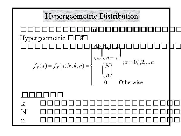
The p. d. of a binomial r. v. If X ~ Bin(n, ), then p(x) = P(X = x) = n. Cx x(1 - )n-x where x = 0, 1, 2, …, n.

Example (Binomial 1) A fair coin is tossed 8 times. Find the probability of obtaining 5 heads. Let X be the number of heads obtained in 8 tosses. Then X ~ Bin(8, 1/2). P(5 heads) = = 7/32

Example (Binomial 2) There are 10 multiple-choice questions in a test and each question has 5 options. Suppose a student answers all 10 questions by randomly picking an option in each question. Find the probability that (a) he will answer six questions correctly, (b) he will get at least 3 correct answers.

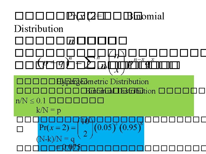
Example (Binomial 2) Let X be the number of correct answers he will get. Then X ~ Bin(10, 0. 2). (a) P(X = 6) = 10 C 6(0. 2)6(1 -0. 2)10 -6 = 0. 00551 (b)P(at least 3 correct answers) = 1 – P(X = 0) – P(X = 1) – P(X = 2) = 1 – 10 C 0(0. 8)10 – 10 C 1(0. 2)(0. 8)9 – 2(0. 8)8 = 0. 322 C (0. 2) 10 2

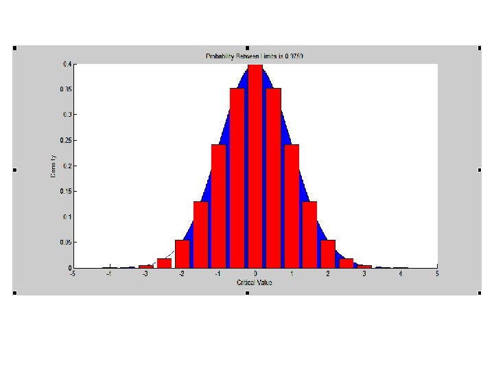
Example (Binomial 3) Binary digits 0 and 1 are transmitted along a data channel in which the presence of noise results in the fact that each digit may be wrongly received with a probabilty of 0. 00002. Each message is transmitted in blocks of 2000 digits. • What is the probabilty that at least one digit in a block is wrongly received? • If a certain message has a length of 20 blocks, find the probability that 2 or more blocks are wrongly received.

Example (Binomial 3) (a) Let X be the number of digits wrongly received in a block of 2000 digits. Then X ~ Bin(2000, 0. 00002). P(X 1)= 1 – P(X = 0) = 1 – 0. 000022000 = 0. 0392

Example (Binomial 3) (b) Let Y be the number of block that are wrongly received among the 20 blocks. Then Y~ Bin(20, 0. 0392). P(Y 2) = 1 – P(Y = 0) – P(Y = 1) = 1 – (1 – 0. 0392)20 – 19 C (0. 0392)(1 – 0. 0392) 20 1 = 0. 184

Normal distribution => A random variable X is said to have a Normal distribution, with parameters and 2 if it can take any real value and has p. d. f. In this case, we write X ~ N( , 2). It can be shown that is the expected value of X and 2 is the variance.

P(a < X < b) = = This integral cannot be done algebraically and its value has to be found by numerical methods of integration. The value of P(a < X < b) can also be viewed as the area under the curve of f(x) from x = a to x = b.

Characteristics of normal distribution 1. 2. 3. 4. Bell shape Symmetric Mean = Mode = Median The 2 tails extend indefinitely

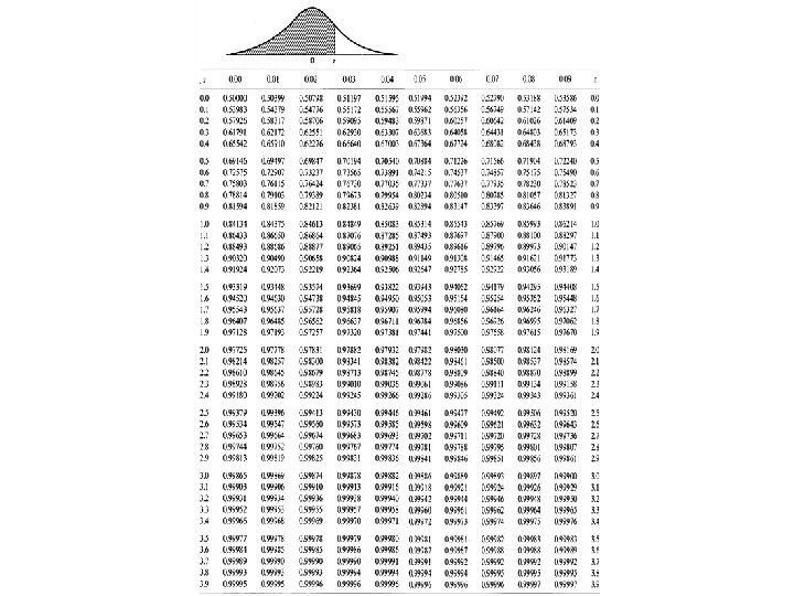
Standard normal distribution A standard normal distribution is the normal distribution with = 0 and 2 = 1, i. e. the N(0, 1) distribution. A standard normal random variable is often denoted by Z. If Z ~ N(0, 1), its c. d. f. is usually written as (z) = P(Z z) =

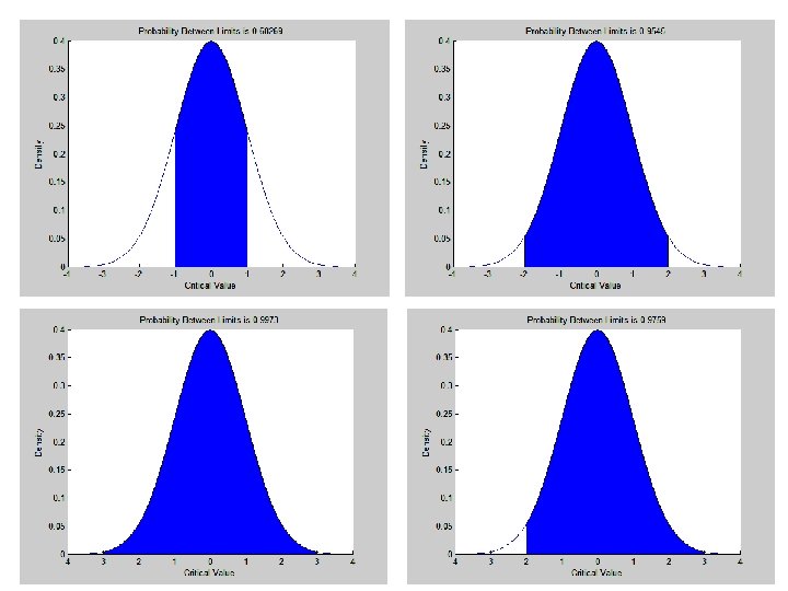
Note: (1) (z) may be interpreted as the area to the left of z under the standard normal curve. (2) P(Z < -z) = P(Z > z), since the standard normal curve is symmetrical about the line Z = 0. (3) The area between Z= -1 and +1 is 68% Z= -2 and +2 is 95% Z= -3 and +3 is 99%

Example => Given Z ~ N(0, 1), find the following probabilities using the standard normal table. (a) p( Z 1. 25) (b) (c) (d) (e) P( Z > 2. 33) P(0. 5 < Z < 1. 5) P( Z < -1. 25) p (-1. 5< Z <-0. 5)

Example (a) P(Z 1. 25) = 0. 8944 (b) P(Z > 2. 33) = 1 - (2. 33) = 1 – 0. 9901 = 0. 0099 (c) P(0. 5 < Z < 1. 5) = (1. 5) - (0. 5) = 0. 9332 – 0. 6915=0. 2417 (d) P( Z < -1. 25) = P(Z > 1. 25) = 1 - (1. 25) = 1 – 0. 8944 = 0. 1056 (e) P(-1. 5 < Z < -0. 5) = 0. 2417

Example (a) P(Z 1. 25) = 0. 8944

Example (b) P(Z > 2. 33) = 1 - (2. 33) = 1 – 0. 9901 = 0. 0099

Example (c) P(0. 5 < Z < 1. 5) = (1. 5) - (0. 5) = 0. 9332 – 0. 6915=0. 2417

Example Given Z ~ N(0, 1), find the value of c if (a) P(Z c) = 0. 8888 (b) P( Z > c) = 0. 37 (c) P(Z < c) = 0. 025 (d) P(0 Z c) = 0. 4924

Example (a) (c) = 0. 8888 c = 1. 22 (b) 1 - (c) = 0. 37 (c) = 0. 63 c = 0. 332

Example (c) Obviously c is negative and the standard normal table cannot be used directly. Recall that P(Z < -z) = P(Z > z) 0. 025 = P(Z < c) = P(Z > -c) = 1 – (-c) = 0. 975 -c = 1. 96 c = -1. 96

Example (d) P(0 Z c) = (c) – 0. 5 = 0. 4924 (c) = 0. 9924 c = 2. 43

Standardization of normal random variables If X ~ N( , 2), then it can be shown that Z= ~ N(0, 1). In other words is the standard normal random variable. The process of transforming X to Z is called standardization of the random variable X.

Example Suppose X ~ N(10, 6. 25). Find the following probabilities (a) P(X < 13) (b) P(X > 5) (c) P(8 < X < 15)

Example Let Z = . (a) P(X < 13) = P(Z < 1. 2) = 0. 8849 )

Example (b) P(X > 5) = P(Z > -2) = P(Z <2) = 0. 9773 )

Example (c) P(8 < X < 15) = P(-0. 8 < Z < 2) = (2) - (-0. 8) = (2) – (1 - (0. 8)) = 0. 9772 – (1 – 0. 7881) = 0. 7653 )