Why I am a Bayesian and why you
Why I am a Bayesian (and why you should become one, too) or Classical statistics considered harmful Kevin Murphy UBC CS & Stats 9 February 2005
Where does the title come from? • “Why I am not a Bayesian”, Glymour, 1981 • “Why Glymour is a Bayesian”, Rosenkrantz, 1983 • “Why isn’t everyone a Bayesian? ”, Efron, 1986 • “Bayesianism and causality, or, why I am only a half-Bayesian”, Pearl, 2001 Many other such philosophical essays…
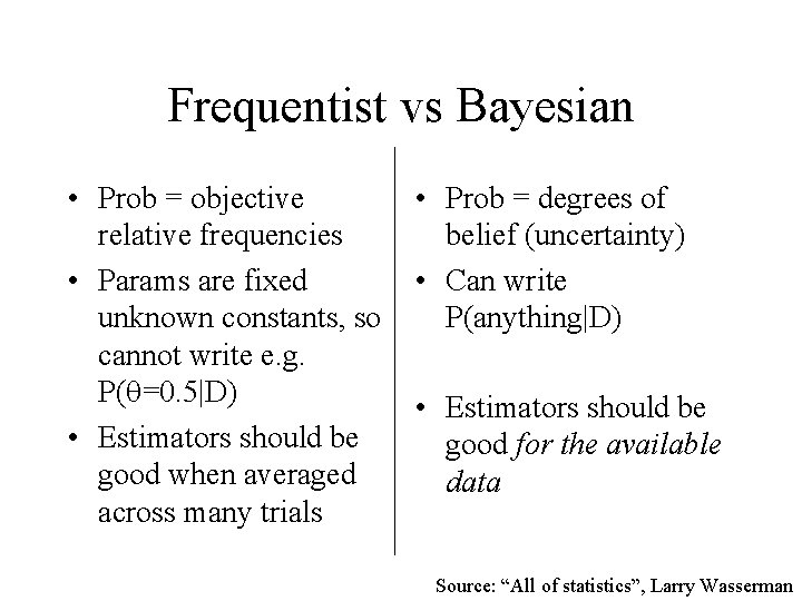
Frequentist vs Bayesian • Prob = objective relative frequencies • Params are fixed unknown constants, so cannot write e. g. P( =0. 5|D) • Estimators should be good when averaged across many trials • Prob = degrees of belief (uncertainty) • Can write P(anything|D) • Estimators should be good for the available data Source: “All of statistics”, Larry Wasserman

Outline • Hypothesis testing – Bayesian approach • Hypothesis testing – classical approach • What’s wrong the classical approach?
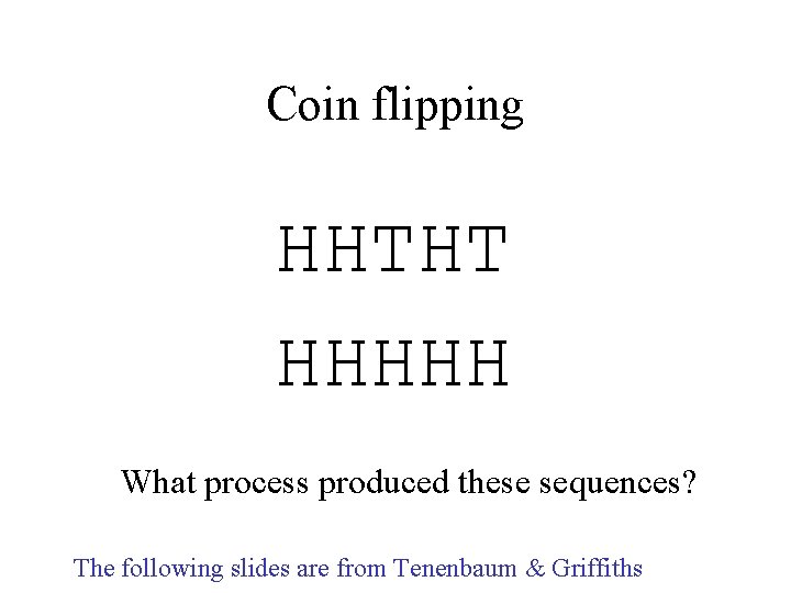
Coin flipping HHTHT HHHHH What process produced these sequences? The following slides are from Tenenbaum & Griffiths
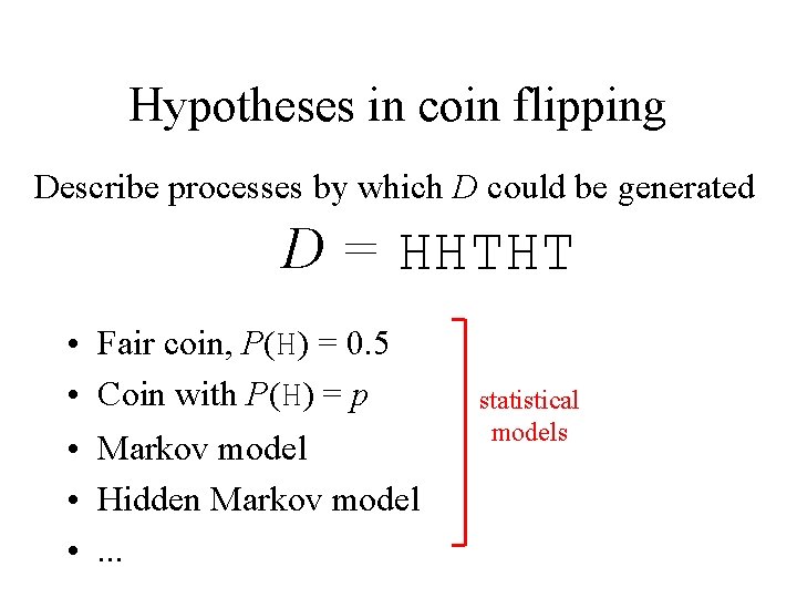
Hypotheses in coin flipping Describe processes by which D could be generated D = HHTHT • Fair coin, P(H) = 0. 5 • Coin with P(H) = p • Markov model • Hidden Markov model • . . . statistical models
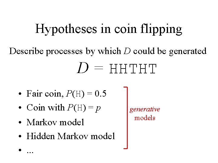
Hypotheses in coin flipping Describe processes by which D could be generated D = HHTHT • Fair coin, P(H) = 0. 5 • Coin with P(H) = p • Markov model • Hidden Markov model • . . . generative models
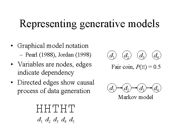
Representing generative models • Graphical model notation – Pearl (1988), Jordan (1998) • Variables are nodes, edges indicate dependency • Directed edges show causal process of data generation HHTHT d 1 d 2 d 3 d 4 d 5 d 1 d 2 d 3 d 4 Fair coin, P(H) = 0. 5 d 1 d 2 d 3 d 4 Markov model
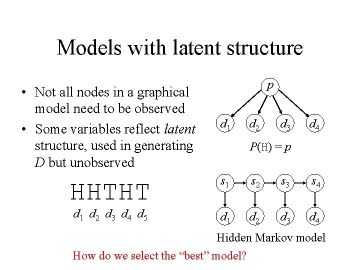
Models with latent structure • Not all nodes in a graphical model need to be observed • Some variables reflect latent structure, used in generating D but unobserved HHTHT d 1 d 2 d 3 d 4 d 5 p d 1 d 2 d 3 d 4 P(H) = p s 1 s 2 s 3 s 4 d 1 d 2 d 3 d 4 Hidden Markov model How do we select the “best” model?
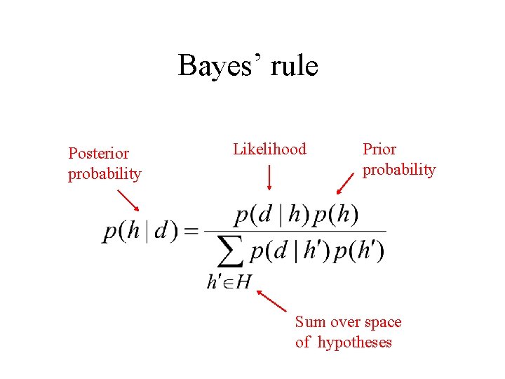
Bayes’ rule Posterior probability Likelihood Prior probability Sum over space of hypotheses
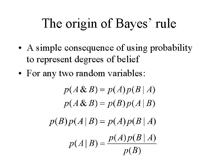
The origin of Bayes’ rule • A simple consequence of using probability to represent degrees of belief • For any two random variables:
Why represent degrees of belief with probabilities? • Good statistics – consistency, and worst-case error bounds. • Cox Axioms – necessary to cohere with common sense • “Dutch Book” + Survival of the Fittest – if your beliefs do not accord with the laws of probability, then you can always be out-gambled by someone whose beliefs do so accord. • Provides a theory of incremental learning – a common currency for combining prior knowledge and the lessons of experience.
Hypotheses in Bayesian inference • Hypotheses H refer to processes that could have generated the data D • Bayesian inference provides a distribution over these hypotheses, given D • P(D|H) is the probability of D being generated by the process identified by H • Hypotheses H are mutually exclusive: only one process could have generated D
Coin flipping • Comparing two simple hypotheses – P(H) = 0. 5 vs. P(H) = 1. 0 • Comparing simple and complex hypotheses – P(H) = 0. 5 vs. P(H) = p
Coin flipping • Comparing two simple hypotheses – P(H) = 0. 5 vs. P(H) = 1. 0 • Comparing simple and complex hypotheses – P(H) = 0. 5 vs. P(H) = p
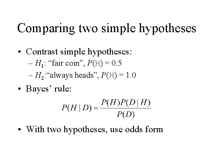
Comparing two simple hypotheses • Contrast simple hypotheses: – H 1: “fair coin”, P(H) = 0. 5 – H 2: “always heads”, P(H) = 1. 0 • Bayes’ rule: • With two hypotheses, use odds form
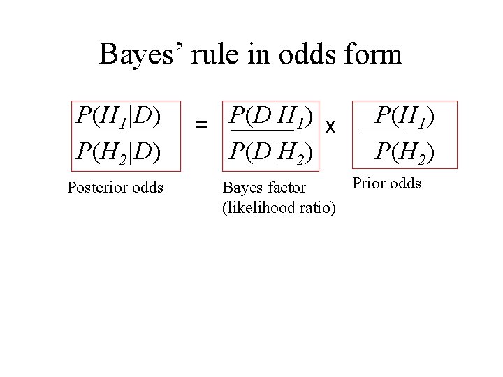
Bayes’ rule in odds form P(H 1|D) P(H 2|D) Posterior odds = P(D|H 1) x P(D|H 2) P(H 1) P(H 2) Prior odds Bayes factor (likelihood ratio)
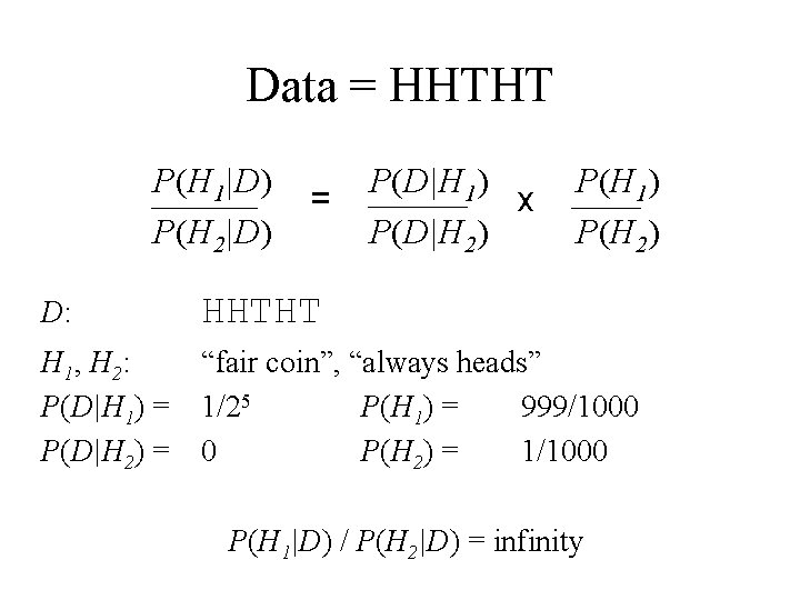
Data = HHTHT P(H 1|D) P(H 2|D) = P(D|H 1) x P(D|H 2) P(H 1) P(H 2) D: HHTHT H 1, H 2: P(D|H 1) = P(D|H 2) = “fair coin”, “always heads” 1/25 P(H 1) = 999/1000 0 P(H 2) = 1/1000 P(H 1|D) / P(H 2|D) = infinity
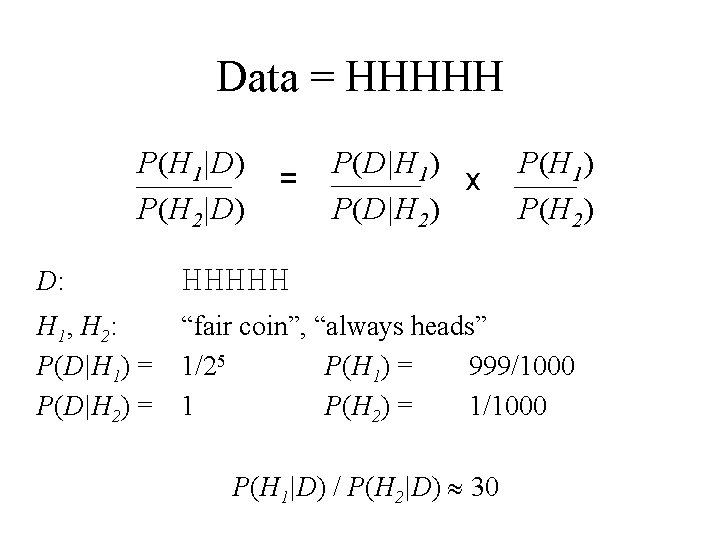
Data = HHHHH P(H 1|D) P(H 2|D) = P(D|H 1) x P(D|H 2) P(H 1) P(H 2) D: HHHHH H 1, H 2: P(D|H 1) = P(D|H 2) = “fair coin”, “always heads” 1/25 P(H 1) = 999/1000 1 P(H 2) = 1/1000 P(H 1|D) / P(H 2|D) 30
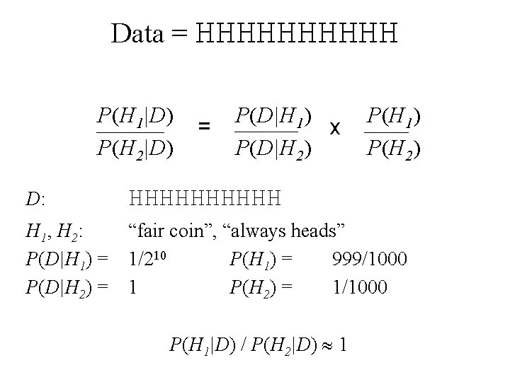
Data = HHHHH P(H 1|D) P(H 2|D) = P(D|H 1) x P(D|H 2) P(H 1) P(H 2) D: HHHHH H 1, H 2: P(D|H 1) = P(D|H 2) = “fair coin”, “always heads” 1/210 P(H 1) = 999/1000 1 P(H 2) = 1/1000 P(H 1|D) / P(H 2|D) 1
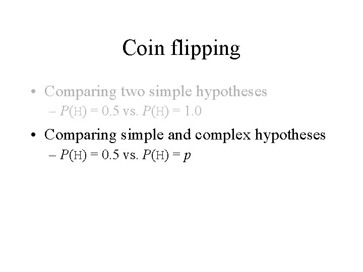
Coin flipping • Comparing two simple hypotheses – P(H) = 0. 5 vs. P(H) = 1. 0 • Comparing simple and complex hypotheses – P(H) = 0. 5 vs. P(H) = p
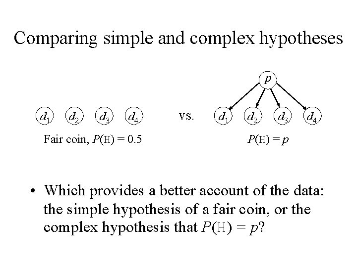
Comparing simple and complex hypotheses p d 1 d 2 d 3 d 4 Fair coin, P(H) = 0. 5 vs. d 1 d 2 d 3 d 4 P(H) = p • Which provides a better account of the data: the simple hypothesis of a fair coin, or the complex hypothesis that P(H) = p?
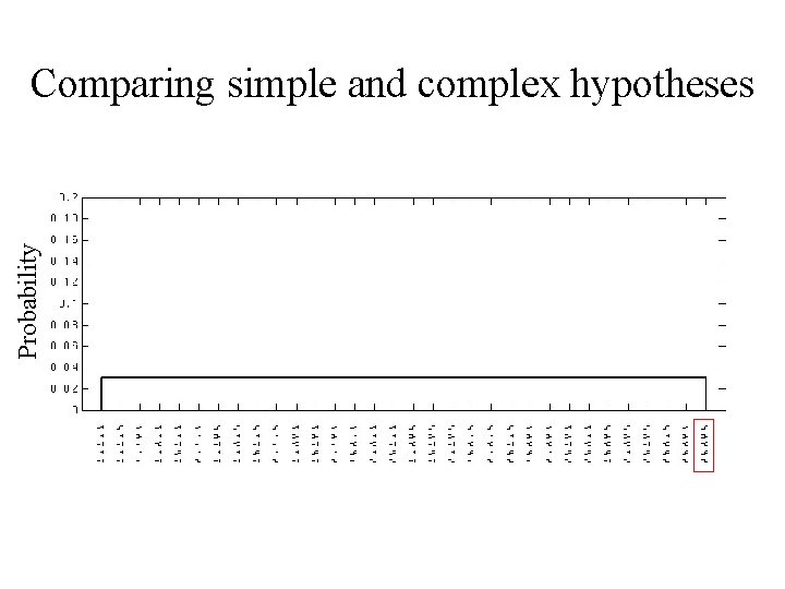
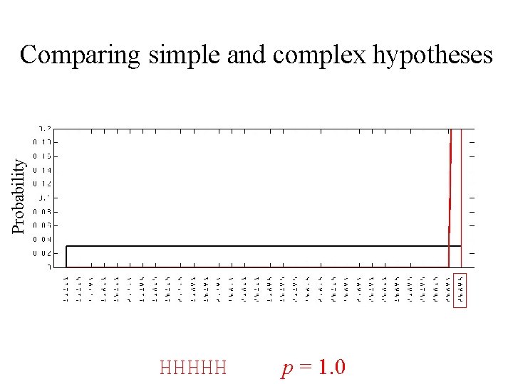
Comparing simple and complex hypotheses • P(H) = p is more complex than P(H) = 0. 5 in two ways: – P(H) = 0. 5 is a special case of P(H) = p – for any observed sequence X, we can choose p such that X is more probable than if P(H) = 0. 5
Probability Comparing simple and complex hypotheses
Probability Comparing simple and complex hypotheses HHHHH p = 1. 0
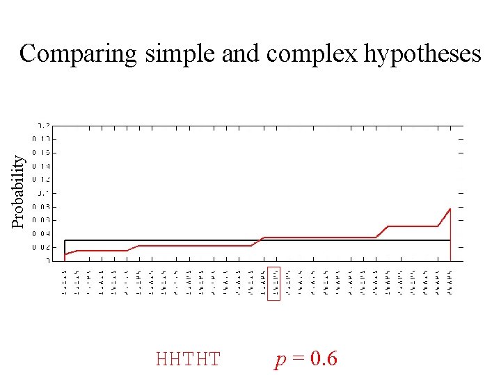
Probability Comparing simple and complex hypotheses HHTHT p = 0. 6
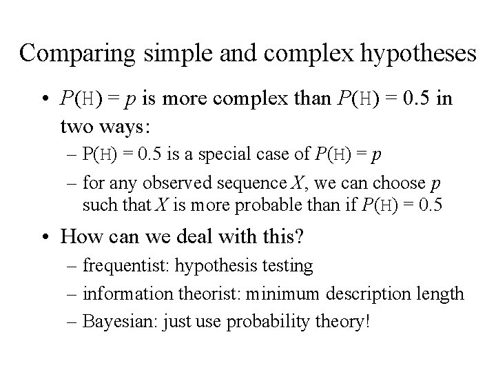
Comparing simple and complex hypotheses • P(H) = p is more complex than P(H) = 0. 5 in two ways: – P(H) = 0. 5 is a special case of P(H) = p – for any observed sequence X, we can choose p such that X is more probable than if P(H) = 0. 5 • How can we deal with this? – frequentist: hypothesis testing – information theorist: minimum description length – Bayesian: just use probability theory!
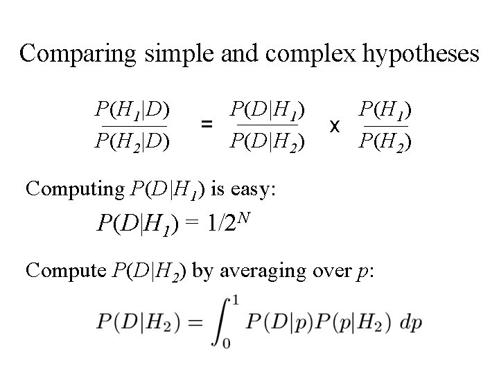
Comparing simple and complex hypotheses P(H 1|D) P(H 2|D) P(D|H 1) = P(D|H 2) P(H 1) x P(H 2) Computing P(D|H 1) is easy: P(D|H 1) = 1/2 N Compute P(D|H 2) by averaging over p:
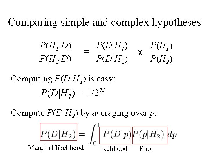
Comparing simple and complex hypotheses P(H 1|D) P(H 2|D) P(D|H 1) = P(D|H 2) P(H 1) x P(H 2) Computing P(D|H 1) is easy: P(D|H 1) = 1/2 N Compute P(D|H 2) by averaging over p: Marginal likelihood Prior
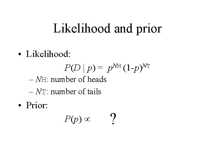
Likelihood and prior • Likelihood: P(D | p) = p. NH (1 -p)NT – NH: number of heads – NT: number of tails • Prior: ? P(p) p. FH-1 (1 -p)FT-1
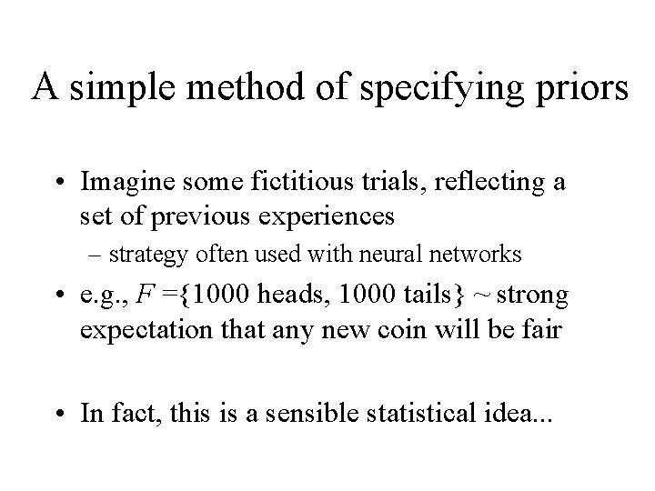
A simple method of specifying priors • Imagine some fictitious trials, reflecting a set of previous experiences – strategy often used with neural networks • e. g. , F ={1000 heads, 1000 tails} ~ strong expectation that any new coin will be fair • In fact, this is a sensible statistical idea. . .
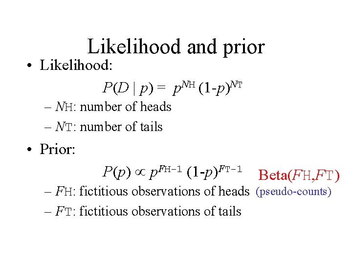
Likelihood and prior • Likelihood: P(D | p) = p. NH (1 -p)NT – NH: number of heads – NT: number of tails • Prior: P(p) p. FH-1 (1 -p)FT-1 Beta(FH, FT) – FH: fictitious observations of heads (pseudo-counts) – FT: fictitious observations of tails
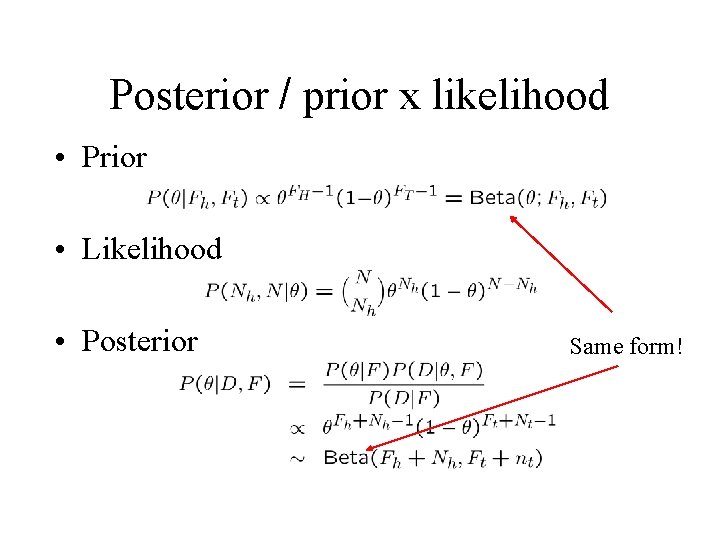
Posterior / prior x likelihood • Prior • Likelihood • Posterior Same form!
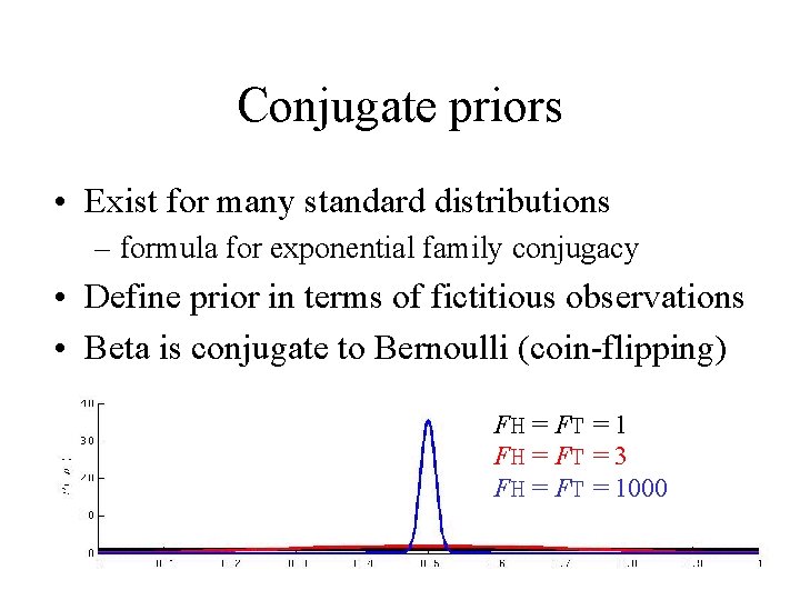
Conjugate priors • Exist for many standard distributions – formula for exponential family conjugacy • Define prior in terms of fictitious observations • Beta is conjugate to Bernoulli (coin-flipping) FH = FT = 1 FH = FT = 3 FH = FT = 1000
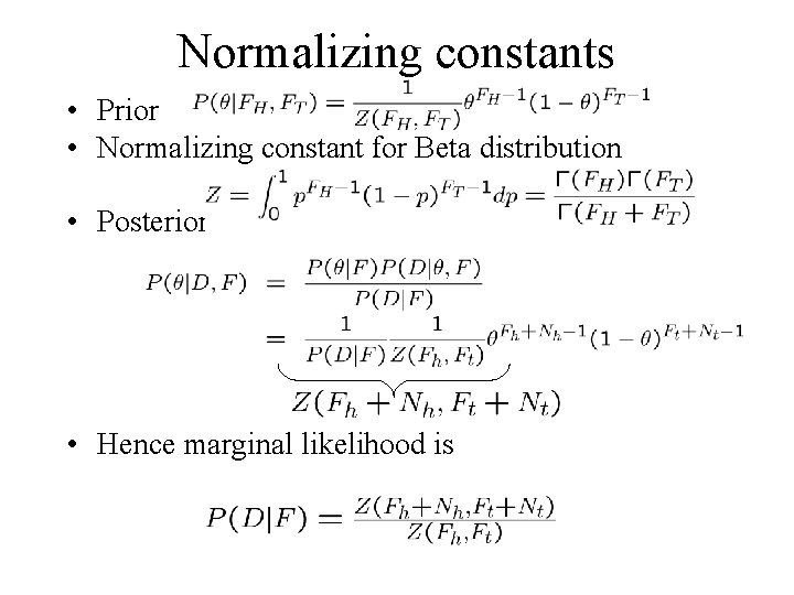
Normalizing constants • Prior • Normalizing constant for Beta distribution • Posterior • Hence marginal likelihood is
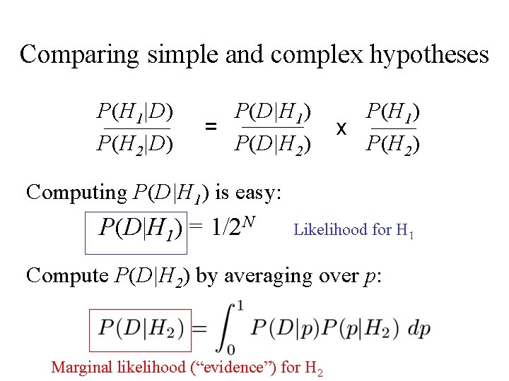
Comparing simple and complex hypotheses P(H 1|D) P(H 2|D) P(D|H 1) = P(D|H 2) P(H 1) x P(H 2) Computing P(D|H 1) is easy: P(D|H 1) = 1/2 N Likelihood for H 1 Compute P(D|H 2) by averaging over p: Marginal likelihood (“evidence”) for H 2
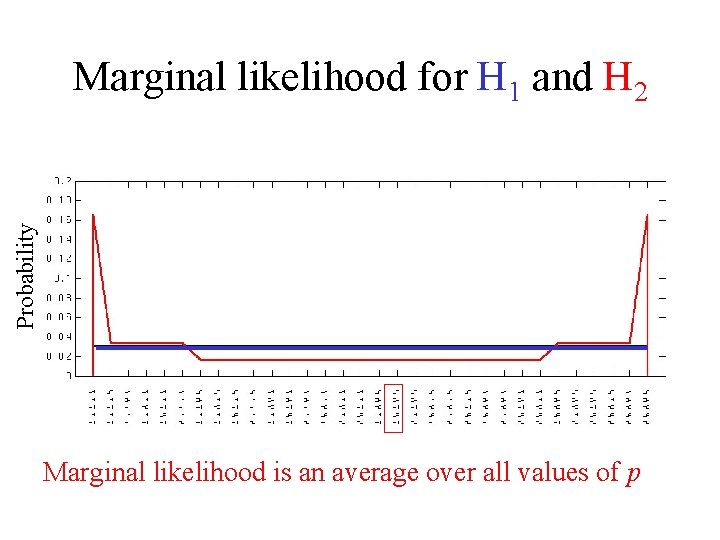
Probability Marginal likelihood for H 1 and H 2 Marginal likelihood is an average over all values of p
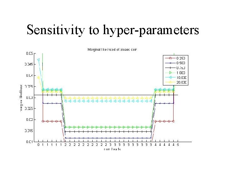
Sensitivity to hyper-parameters
Bayesian model selection • Simple and complex hypotheses can be compared directly using Bayes’ rule – requires summing over latent variables • Complex hypotheses are penalized for their greater flexibility: “Bayesian Occam’s razor” • Maximum likelihood cannot be used for model selection (always prefers hypothesis with largest number of parameters)
Outline • Hypothesis testing – Bayesian approach • Hypothesis testing – classical approach • What’s wrong the classical approach?
Example: Belgian euro-coins • A Belgian euro spun N=250 times came up heads X=140. • “It looks very suspicious to me. If the coin were unbiased the chance of getting a result as extreme as that would be less than 7%” – Barry Blight, LSE (reported in Guardian, 2002) Source: Mackay exercise 3. 15
Classical hypothesis testing • Null hypothesis H 0 eg. = 0. 5 (unbiased coin) • For classical analysis, don’t need to specify alternative hypothesis, but later we will use H 1: 0. 5 • Need a decision rule that maps data D to accept/ reject of H 0. • Define a scalar measure of deviance d(D) from the null hypothesis e. g. , Nh or 2
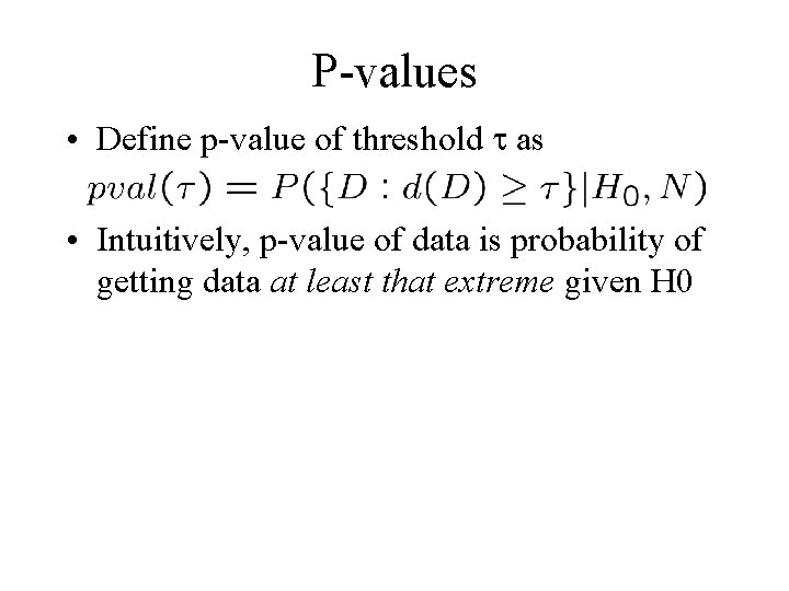
P-values • Define p-value of threshold as • Intuitively, p-value of data is probability of getting data at least that extreme given H 0
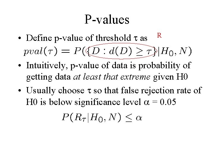
P-values • Define p-value of threshold as R • Intuitively, p-value of data is probability of getting data at least that extreme given H 0 • Usually choose so that false rejection rate of H 0 is below significance level = 0. 05
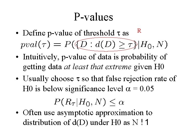
P-values • Define p-value of threshold as R • Intuitively, p-value of data is probability of getting data at least that extreme given H 0 • Usually choose so that false rejection rate of H 0 is below significance level = 0. 05 • Often use asymptotic approximation to distribution of d(D) under H 0 as N ! 1
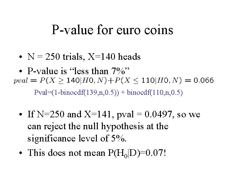
P-value for euro coins • N = 250 trials, X=140 heads • P-value is “less than 7%” Pval=(1 -binocdf(139, n, 0. 5)) + binocdf(110, n, 0. 5) • If N=250 and X=141, pval = 0. 0497, so we can reject the null hypothesis at the significance level of 5%. • This does not mean P(H 0|D)=0. 07!
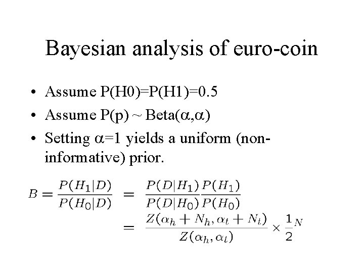
Bayesian analysis of euro-coin • Assume P(H 0)=P(H 1)=0. 5 • Assume P(p) ~ Beta( , ) • Setting =1 yields a uniform (noninformative) prior.
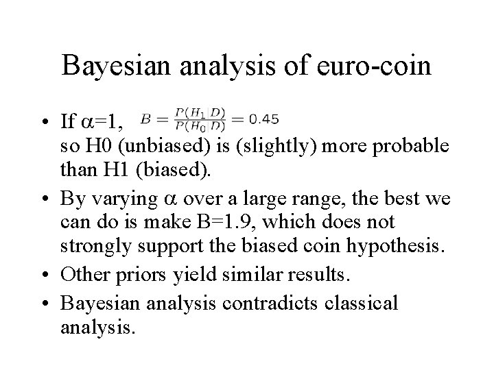
Bayesian analysis of euro-coin • If =1, so H 0 (unbiased) is (slightly) more probable than H 1 (biased). • By varying over a large range, the best we can do is make B=1. 9, which does not strongly support the biased coin hypothesis. • Other priors yield similar results. • Bayesian analysis contradicts classical analysis.
Outline • Hypothesis testing – Bayesian approach • Hypothesis testing – classical approach • What’s wrong the classical approach?
Outline • Hypothesis testing – Bayesian approach • Hypothesis testing – classical approach • What’s wrong the classical approach? – Violates likelihood principle – Violates stopping rule principle – Violates common sense
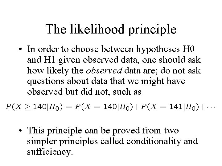
The likelihood principle • In order to choose between hypotheses H 0 and H 1 given observed data, one should ask how likely the observed data are; do not ask questions about data that we might have observed but did not, such as • This principle can be proved from two simpler principles called conditionality and sufficiency.
Frequentist statistics violates the likelihood principle • “The use of P-values implies that a hypothesis that may be true can be rejected because it has not predicted observable results that have not actually occurred. ” – Jeffreys, 1961
Another example • • Suppose X ~ N( , 2); we observe x=3 Compare H 0: =0 with H 1: >0 P-value = P(X ¸ 3|H 0)=0. 001, so reject H 0 Bayesian approach: update P( |X) using conjugate analysis; compute Bayes factor to compare H 0 and H 1
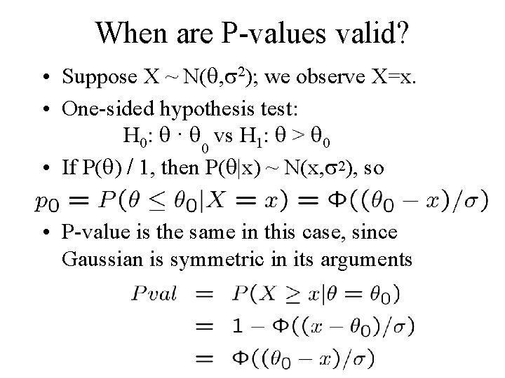
When are P-values valid? • Suppose X ~ N( , 2); we observe X=x. • One-sided hypothesis test: H 0: · 0 vs H 1: > 0 • If P( ) / 1, then P( |x) ~ N(x, 2), so • P-value is the same in this case, since Gaussian is symmetric in its arguments
Outline • Hypothesis testing – Bayesian approach • Hypothesis testing – classical approach • What’s wrong the classical approach? – Violates likelihood principle – Violates stopping rule principle – Violates common sense
Stopping rule principle • Inferences you make should only depend on the observed data, not the reasons why this data was collected. • If you look at your data to decide when to stop collecting, this should not change any conclusions you draw. • Follows from likelihood principle.
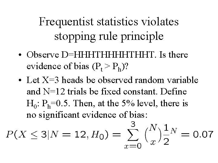
Frequentist statistics violates stopping rule principle • Observe D=HHHTHHT. Is there evidence of bias (Pt > Ph)? • Let X=3 heads be observed random variable and N=12 trials be fixed constant. Define H 0: Ph=0. 5. Then, at the 5% level, there is no significant evidence of bias:
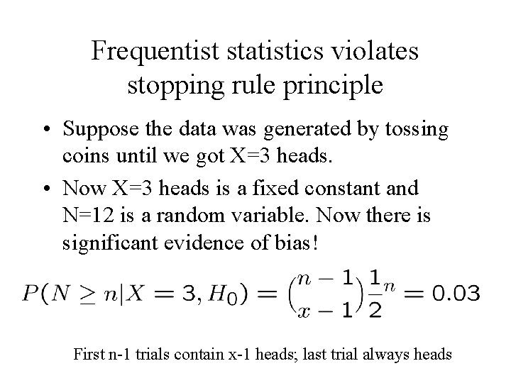
Frequentist statistics violates stopping rule principle • Suppose the data was generated by tossing coins until we got X=3 heads. • Now X=3 heads is a fixed constant and N=12 is a random variable. Now there is significant evidence of bias! First n-1 trials contain x-1 heads; last trial always heads
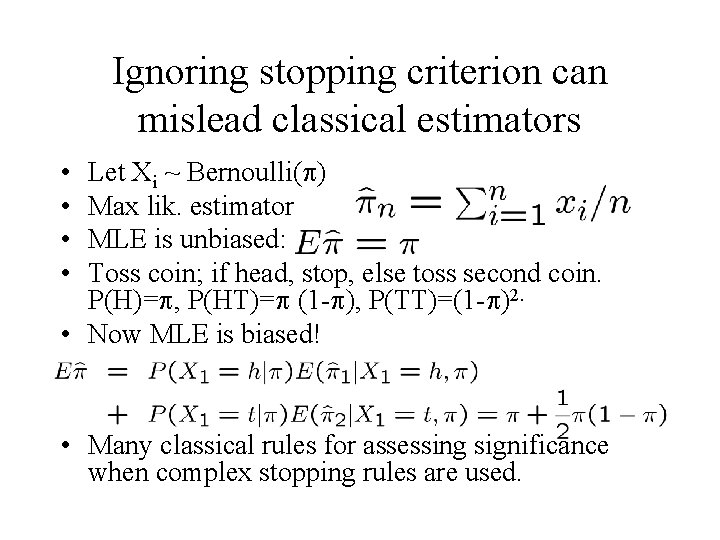
Ignoring stopping criterion can mislead classical estimators • • Let Xi ~ Bernoulli( ) Max lik. estimator MLE is unbiased: Toss coin; if head, stop, else toss second coin. P(H)= , P(HT)= (1 - ), P(TT)=(1 - )2. • Now MLE is biased! • Many classical rules for assessing significance when complex stopping rules are used.
Outline • Hypothesis testing – Bayesian approach • Hypothesis testing – classical approach • What’s wrong the classical approach? – Violates likelihood principle – Violates stopping rule principle – Violates common sense
Confidence intervals • An interval ( min(D), max(D)) is a 95% CI if lies inside this interval 95% of the time across repeated draws D~P(. | ) • This does not mean P( 2 CI|D) = 0. 95! Mackay sec 37. 3
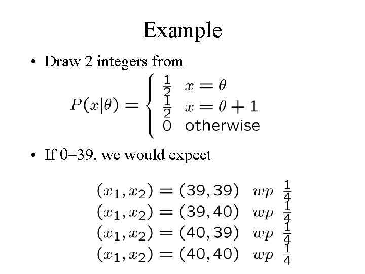
Example • Draw 2 integers from • If =39, we would expect
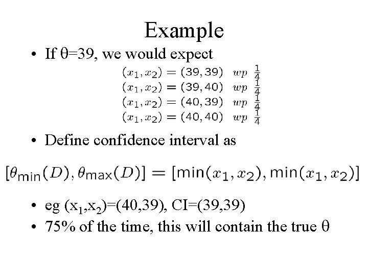
Example • If =39, we would expect • Define confidence interval as • eg (x 1, x 2)=(40, 39), CI=(39, 39) • 75% of the time, this will contain the true
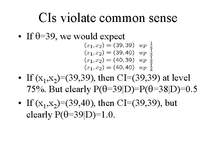
CIs violate common sense • If =39, we would expect • If (x 1, x 2)=(39, 39), then CI=(39, 39) at level 75%. But clearly P( =39|D)=P( =38|D)=0. 5 • If (x 1, x 2)=(39, 40), then CI=(39, 39), but clearly P( =39|D)=1. 0.
What’s wrong with the classical approach? • Violates likelihood principle • Violates stopping rule principle • Violates common sense
What’s right about the Bayesian approach? • Simple and natural • Optimal mechanism for reasoning under uncertainty • Generalization of Aristotelian logic that reduces to deductive logic if our hypotheses are either true or false • Supports interesting (human-like) kinds of learning

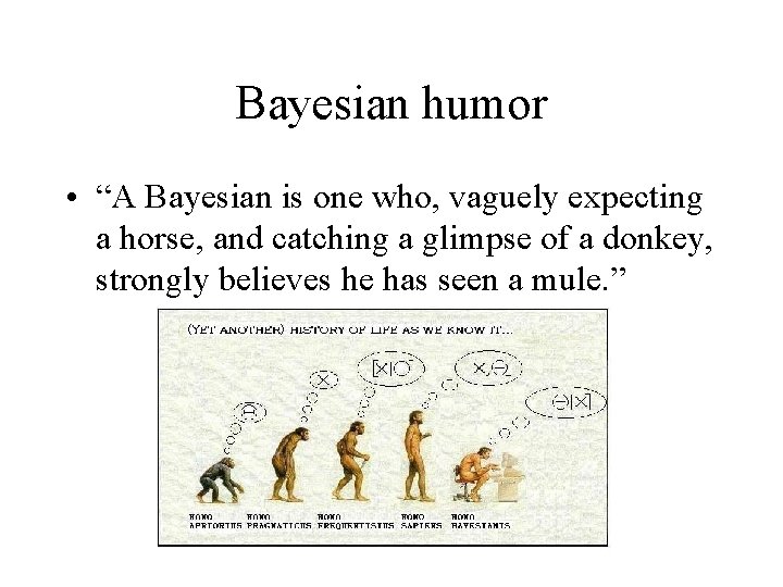
Bayesian humor • “A Bayesian is one who, vaguely expecting a horse, and catching a glimpse of a donkey, strongly believes he has seen a mule. ”
- Slides: 68