Why have sex The population genetics of sex

Why have sex? The population genetics of sex and recombination Sally Otto Department of Zoology University of British Columbia

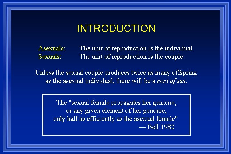
INTRODUCTION Asexuals: Sexuals: The unit of reproduction is the individual The unit of reproduction is the couple Unless the sexual couple produces twice as many offspring as the asexual individual, there will be a cost of sex. The "sexual female propagates her genome, or any given element of her genome, only half as efficiently as the asexual female" — Bell 1982

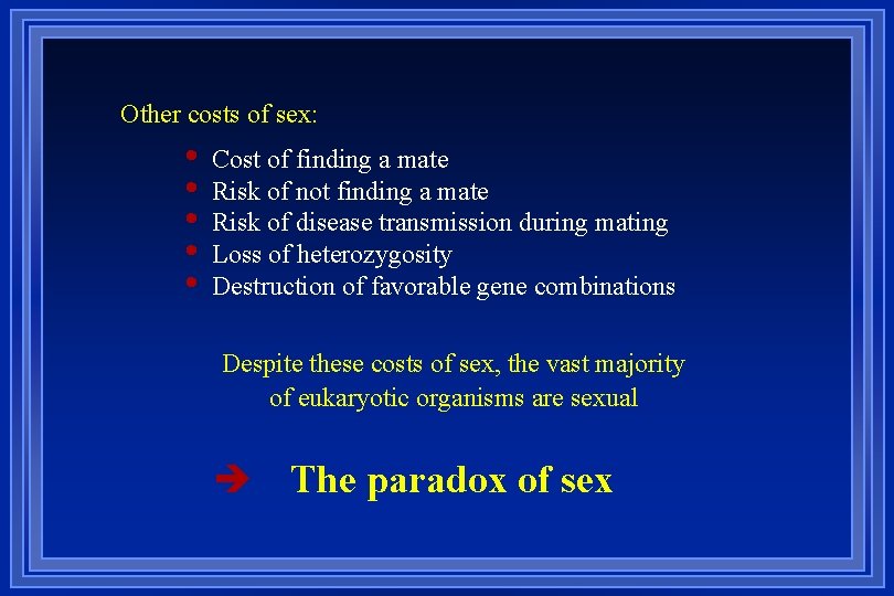
Other costs of sex: • • • Cost of finding a mate Risk of not finding a mate Risk of disease transmission during mating Loss of heterozygosity Destruction of favorable gene combinations Despite these costs of sex, the vast majority of eukaryotic organisms are sexual è The paradox of sex

What might offset the cost of sex? • Paternal contribution to the production and rearing of offspring What might pay the cost of sex? • Most explanations of sex stem from the idea that sex can generate greater variability through chromosomal segregation and recombination.

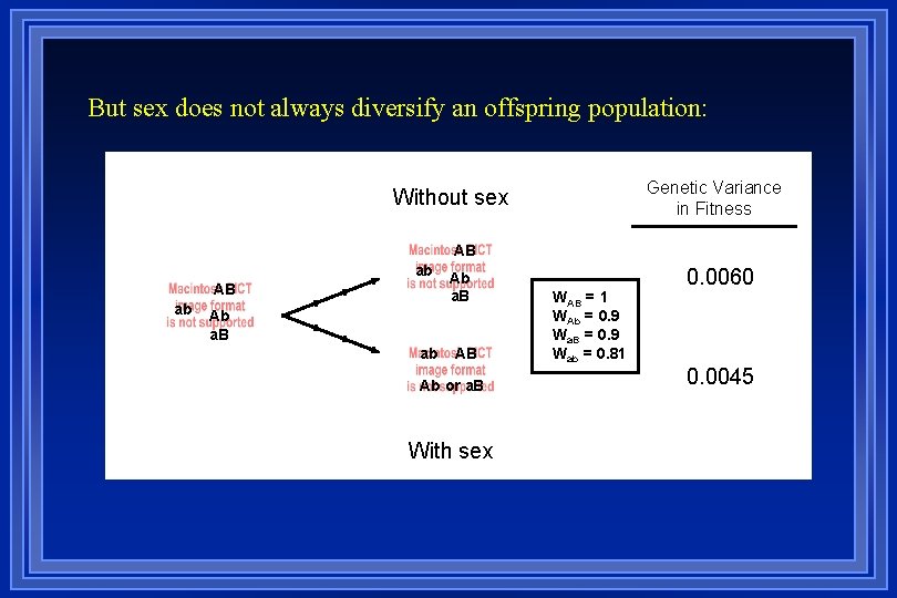
But sex does not always diversify an offspring population: Genetic Variance in Fitness Without sex AB ab Ab a. B ab AB Ab or a. B With sex WAB = 1 WAb = 0. 9 Wa. B = 0. 9 Wab = 0. 81 0. 0060 0. 0045

An increase in genetic variation (Vg) generally improves the response of a population to selection. • Identify the conditions under which sex and recombination increase genetic variation • Determine the extent to which this force favors the evolution of sex and recombination

Genotypes that are more common than expected based on Hardy-Weinberg or linkage equilibrium are typically more common because they have been favored by selection. By destroying these genetic associations, sex and recombination typically reduce the average fitness of offspring. è RECOMBINATION LOAD

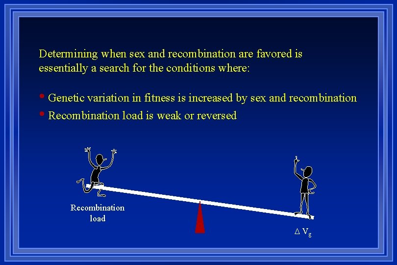
Determining when sex and recombination are favored is essentially a search for the conditions where: • Genetic variation in fitness is increased by sex and recombination • Recombination load is weak or reversed Recombination load D Vg

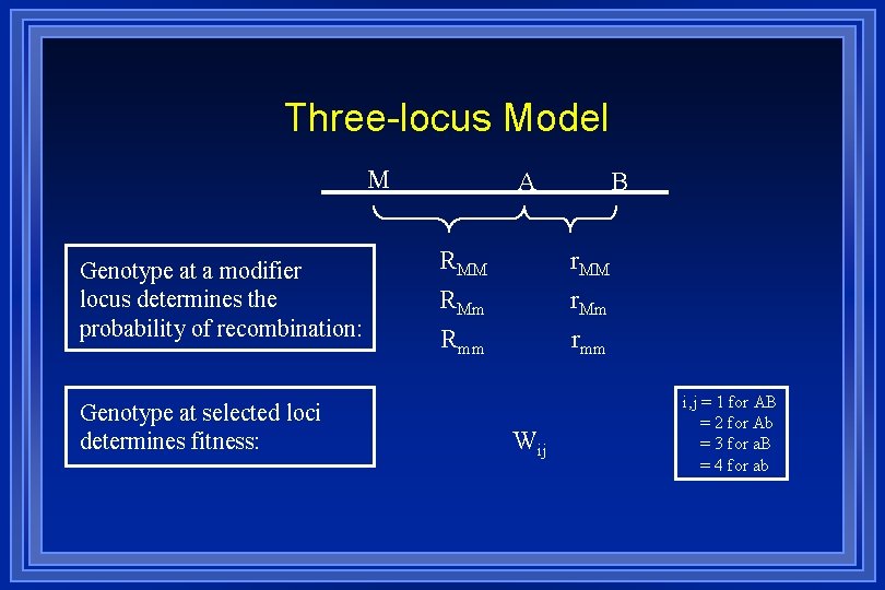
Three-locus Model M Genotype at a modifier locus determines the probability of recombination: Genotype at selected loci determines fitness: A RMM RMm Rmm B r. MM r. Mm rmm Wij i, j = 1 for AB = 2 for Ab = 3 for a. B = 4 for ab

ASIDE: Are sex and recombination interchangeable? ? ? In general, NO, because sex involves both segregation and recombination. è Segregation at one locus can exert selection for/against sex (Kirkpatrick and Jenkins 1989; Chasnov 2000; Agrawal 2001*) In haploid models, however, the probability of sex and the probability of recombination enter into models as their product. (True also for special diploid models where HW is maintained by selection. ) è Models that examine the fate of alleles that modify recombination rates inform us about the fate of alleles that modify the probability of engaging in sex.

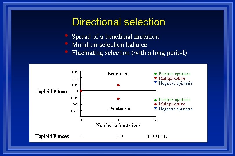
Directional selection • • • Spread of a beneficial mutation Mutation-selection balance Fluctuating selection (with a long period) 1. 75 Beneficial 1. 5 Positive epistasis Multiplicative Negative epistasis 1. 25 Haploid Fitness 1 0. 75 Positive epistasis Multiplicative Negative epistasis ] 0. 5 Deleterious 0. 25 0 1 2 Number of mutations Haploid Fitness: 1 1+s (1+s)2+e

Initial Population 0. 4 D=0 0. 3 0. 2 0. 1 AB Ab e<0 ab e=0 D<0 0. 4 a. B D=0 0. 4 e>0 0. 3 0. 2 0. 1 AB Ab a. B ab AB Ab a. B D>0 0. 4 ab AB Ab a. B ab

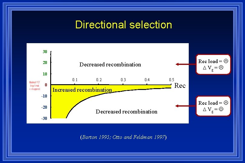
Directional selection 30 20 Rec load = D Vg = Decreased recombination 10 0. 1 0 0. 2 0. 3 0. 4 Increased recombination 0. 5 Rec -10 -20 Decreased recombination -30 (Barton 1995; Otto and Feldman 1997) Rec load = D Vg =

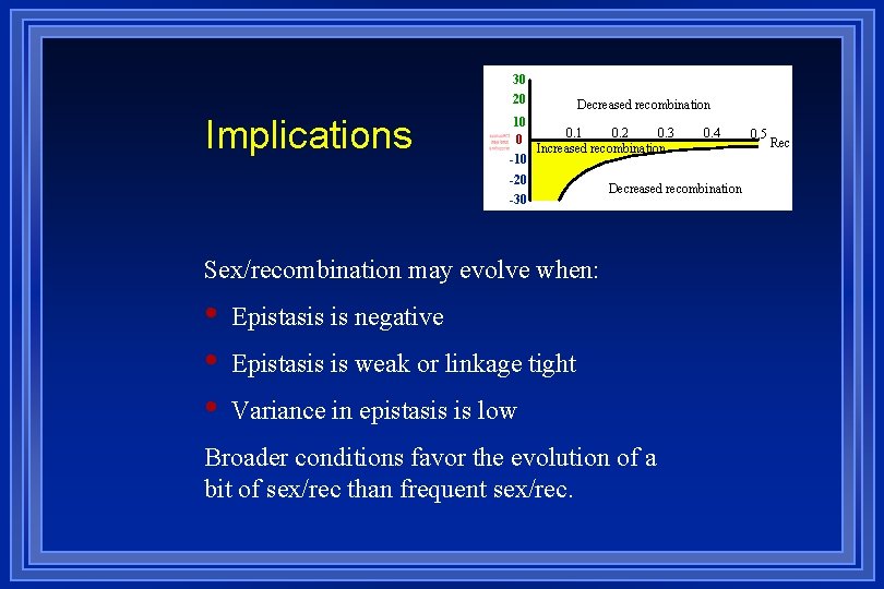
30 20 Implications 10 0 -10 Decreased recombination 0. 1 0. 2 0. 3 Increased recombination -20 -30 Decreased recombination Sex/recombination may evolve when: • • • 0. 4 Epistasis is negative Epistasis is weak or linkage tight Variance in epistasis is low Broader conditions favor the evolution of a bit of sex/rec than frequent sex/rec. 0. 5 Rec

Less restrictive explanations? ? ? Temporal variation in selection (e. g. host-parasite mediated): • Disequilibrium may reflect past not current selection è Sex/recombination can gain an immediate fitness benefit by breaking down disequilibrium • Rec load = But fluctuations have to be very rapid (2~5 generations) (Barton 1995; Peters and Lively 1999)

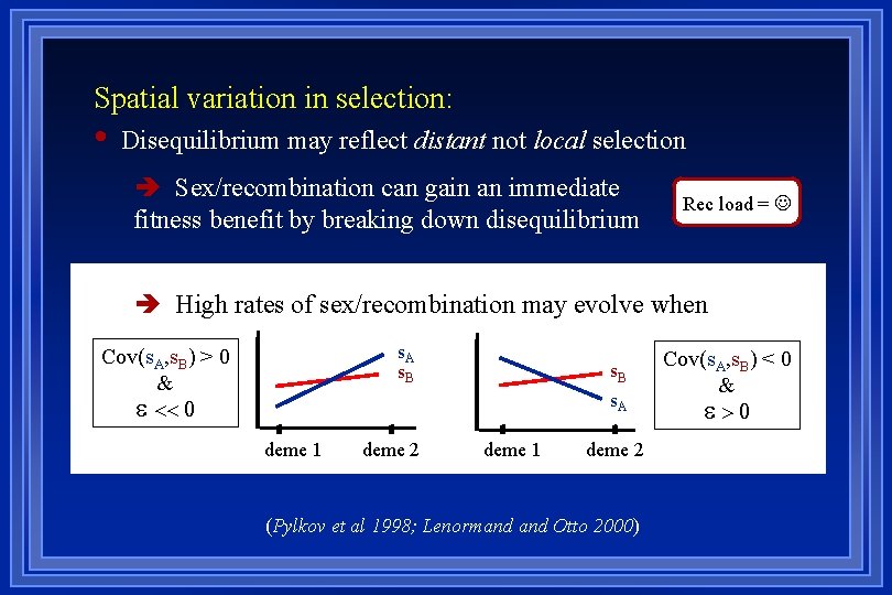
Spatial variation in selection: • Disequilibrium may reflect distant not local selection è Sex/recombination can gain an immediate fitness benefit by breaking down disequilibrium Rec load = è High rates of sex/recombination may evolve when s. A s. B Cov(s. A, s. B) > 0 & e << 0 deme 1 deme 2 / s. B s. A deme 1 deme 2 (Pylkov et al 1998; Lenormand Otto 2000) Cov(s. A, s. B) < 0 & e>0

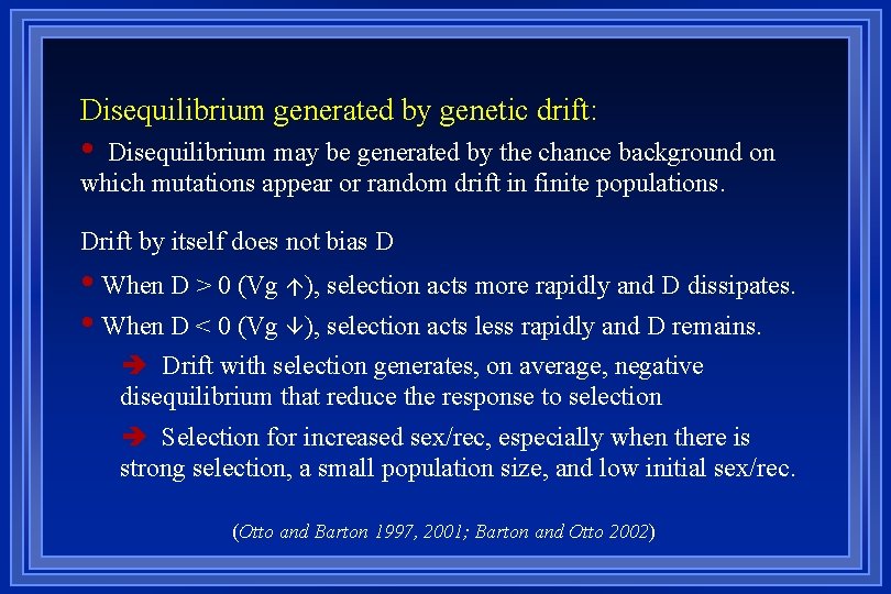
Disequilibrium generated by genetic drift: • Disequilibrium may be generated by the chance background on which mutations appear or random drift in finite populations. Drift by itself does not bias D • When D > 0 (Vg ), selection acts more rapidly and D dissipates. • When D < 0 (Vg ), selection acts less rapidly and D remains. è Drift with selection generates, on average, negative disequilibrium that reduce the response to selection è Selection for increased sex/rec, especially when there is strong selection, a small population size, and low initial sex/rec. (Otto and Barton 1997, 2001; Barton and Otto 2002)

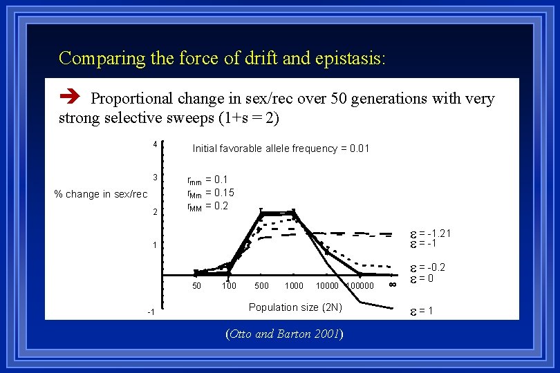
Comparing the force of drift and epistasis: è Proportional change in sex/rec over 50 generations with very strong selective sweeps (1+s = 2) 4 3 % change in sex/rec 2 Initial favorable allele frequency = 0. 01 rmm = 0. 1 r. Mm = 0. 15 r. MM = 0. 2 / e = -1. 21 e = -1 1 50 -1 100 500 100000 Population size (2 N) (Otto and Barton 2001) e = -0. 2 =0 ∞ e e=1

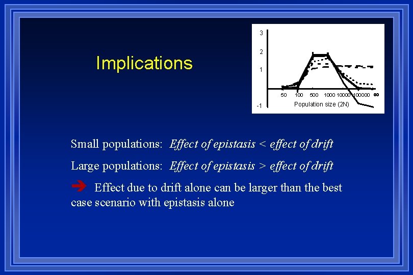
3 Implications 2 / 1 50 -1 100 500 100000 Population size (2 N) Small populations: Effect of epistasis < effect of drift Large populations: Effect of epistasis > effect of drift è Effect due to drift alone can be larger than the best case scenario with epistasis alone ∞

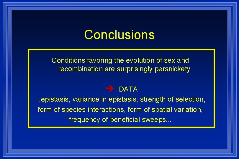
Conclusions Conditions favoring the evolution of sex and recombination are surprisingly persnickety è DATA. . . epistasis, variance in epistasis, strength of selection, form of species interactions, form of spatial variation, frequency of beneficial sweeps. . .