Where weve been where were going We can

Where we’ve been & where we’re going We can use data to address following questions: 1. Question: Is a mean = some number? Large sample z-test and CI Small sample t-test and CI 2. Question: Is a proportion = some %? Proportion version of large sample z-test and CI

Where we’ve been & where we’re going 3. Question: 4. Question: Is a diff between two means = some # Independent samples: large sample z test and CI small sample t test and CI paired samples: small sample paired t test and CI Is diff between 2 proportions = some % Proportion version of large sample z test and CI

Topics to be covered in remaining 8 classes (including today) Analysis of Variance and Linear Regression (Chapters 11, 12 and 13) “response = b 0 + b 1 covariate 1 + … +bp covariate p + error” Categorical Data / Contingency Tables “when response is discrete…”

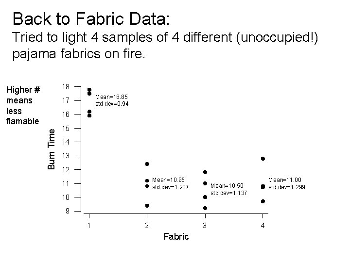
Back to Fabric Data: Tried to light 4 samples of 4 different (unoccupied!) pajama fabrics on fire. 18 Higher # means less flamable Mean=16. 85 std dev=0. 94 17 Burn Time 16 15 14 13 12 Mean=10. 95 std dev=1. 237 11 Mean=11. 00 std dev=1. 299 Mean=10. 50 std dev=1. 137 10 9 1 2 3 Fabric 4

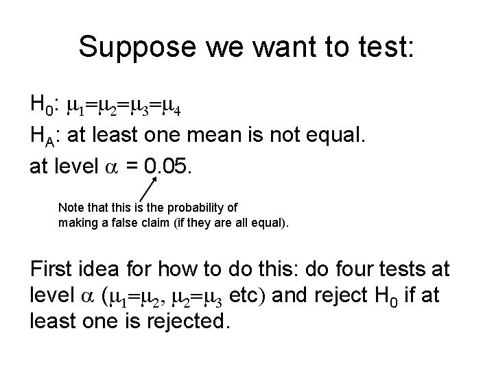
Suppose we want to test: H 0: m 1=m 2=m 3=m 4 HA: at least one mean is not equal. at level a = 0. 05. Note that this is the probability of making a false claim (if they are all equal). First idea for how to do this: do four tests at level a (m 1=m 2, m 2=m 3 etc) and reject H 0 if at least one is rejected.

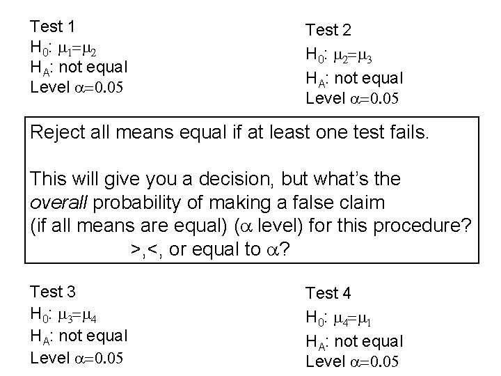
Test 1 H 0: m 1=m 2 HA: not equal Level a=0. 05 Test 2 H 0: m 2=m 3 HA: not equal Level a=0. 05 Reject all means equal if at least one test fails. This will give you a decision, but what’s the overall probability of making a false claim (if all means are equal) (a level) for this procedure? >, <, or equal to a? Test 3 H 0: m 3=m 4 HA: not equal Level a=0. 05 Test 4 H 0: m 4=m 1 HA: not equal Level a=0. 05

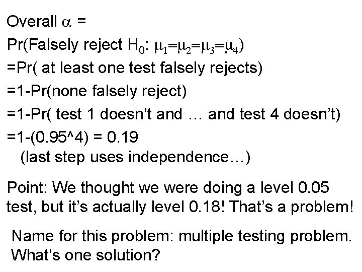
Overall a = Pr(Falsely reject H 0: m 1=m 2=m 3=m 4) =Pr( at least one test falsely rejects) =1 -Pr(none falsely reject) =1 -Pr( test 1 doesn’t and … and test 4 doesn’t) =1 -(0. 95^4) = 0. 19 (last step uses independence…) Point: We thought we were doing a level 0. 05 test, but it’s actually level 0. 18! That’s a problem! Name for this problem: multiple testing problem. What’s one solution?

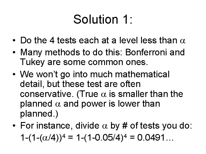
Solution 1: • Do the 4 tests each at a level less than a • Many methods to do this: Bonferroni and Tukey are some common ones. • We won’t go into much mathematical detail, but these test are often conservative. (True a is smaller than the planned a and power is lower than planned. ) • For instance, divide a by # of tests you do: 1 -(1 -(a/4))4 = 1 -(1 -0. 05/4)4 = 0. 0491…

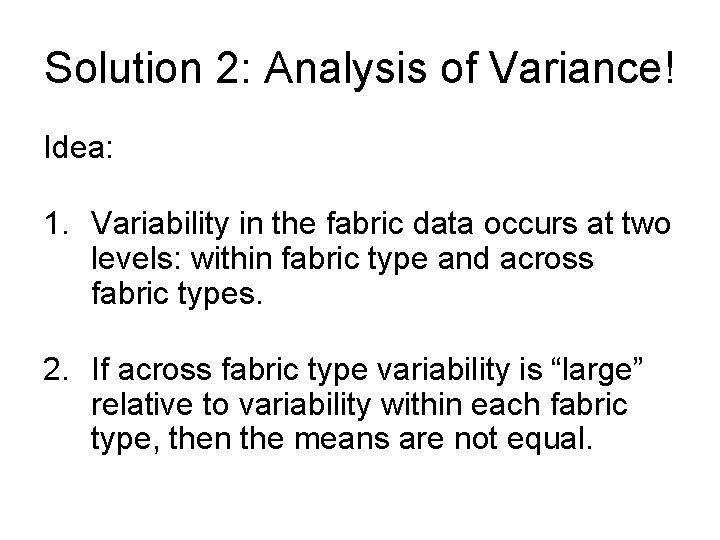
Solution 2: Analysis of Variance! Idea: 1. Variability in the fabric data occurs at two levels: within fabric type and across fabric types. 2. If across fabric type variability is “large” relative to variability within each fabric type, then the means are not equal.

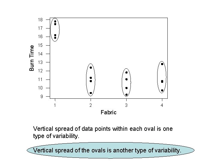
18 17 Burn Time 16 15 14 13 12 11 10 9 1 2 3 4 Fabric Vertical spread of data points within each oval is one type of variability. Vertical spread of the ovals is another type of variability.

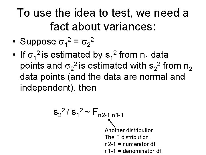
To use the idea to test, we need a fact about variances: • Suppose s 12 = s 22 • If s 12 is estimated by s 12 from n 1 data points and s 22 is estimated with s 22 from n 2 data points (and the data are normal and independent), then s 22 / s 12 ~ Fn 2 -1, n 1 -1 Another distribution. The F distribution. n 2 -1 = numerator df n 1 -1 = denominator df

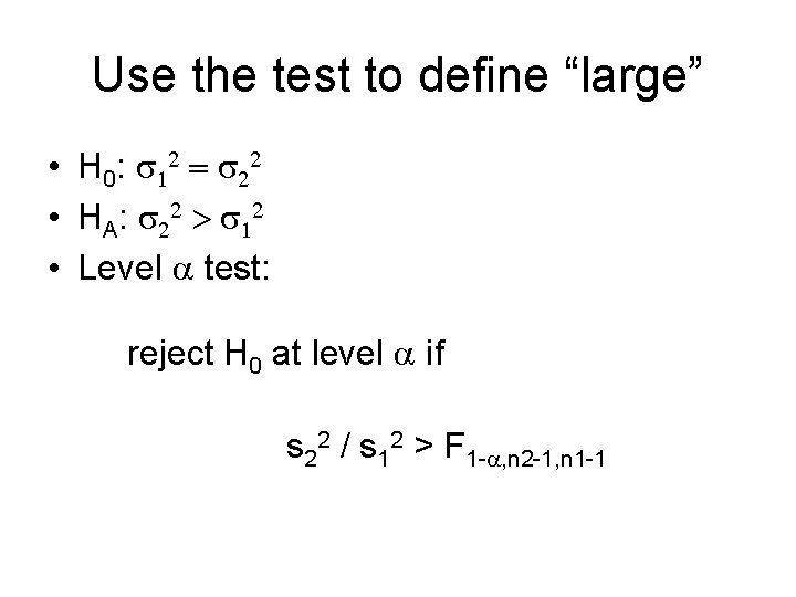
Use the test to define “large” • H 0: s 12 = s 22 • HA: s 22 > s 12 • Level a test: reject H 0 at level a if s 22 / s 12 > F 1 -a, n 2 -1, n 1 -1

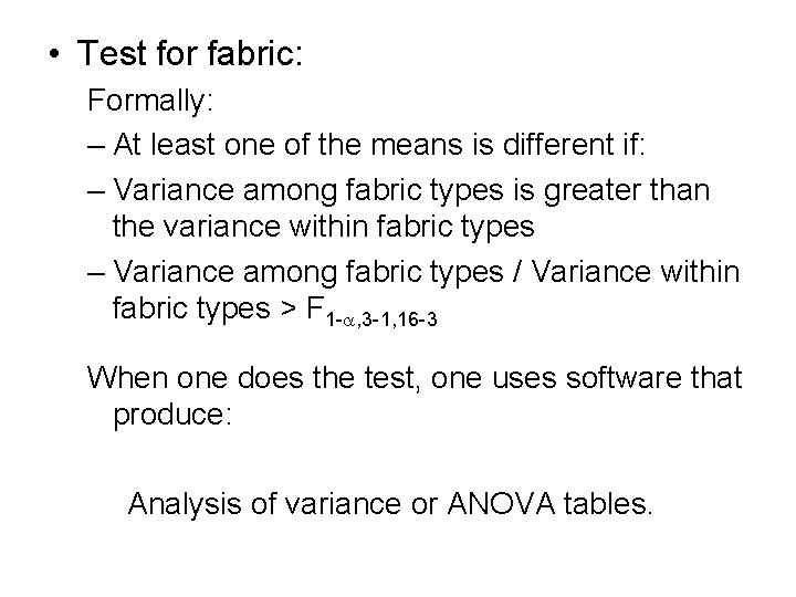
• Test for fabric: Formally: – At least one of the means is different if: – Variance among fabric types is greater than the variance within fabric types – Variance among fabric types / Variance within fabric types > F 1 -a, 3 -1, 16 -3 When one does the test, one uses software that produce: Analysis of variance or ANOVA tables.

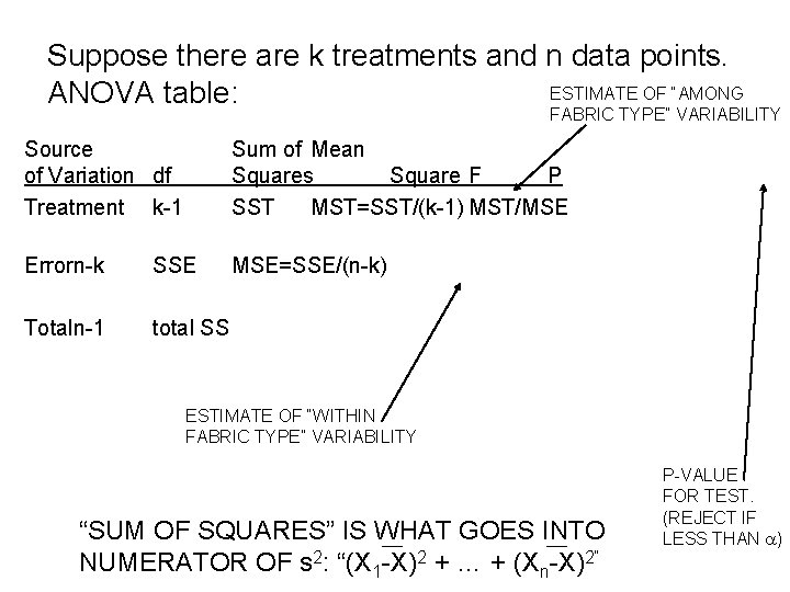
Suppose there are k treatments and n data points. ESTIMATE OF “AMONG ANOVA table: FABRIC TYPE” VARIABILITY Source of Variation df Treatment k-1 Sum of Mean Squares Square F P SST MST=SST/(k-1) MST/MSE Errorn-k SSE MSE=SSE/(n-k) Totaln-1 total SS ESTIMATE OF “WITHIN FABRIC TYPE” VARIABILITY “SUM OF SQUARES” IS WHAT GOES INTO NUMERATOR OF s 2: “(X 1 -X)2 + … + (Xn-X)2” P-VALUE FOR TEST. (REJECT IF LESS THAN a)

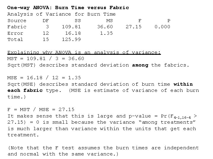
One-way ANOVA: Burn Time versus Fabric Analysis of Variance for Burn Time Source DF SS MS F Fabric 3 109. 81 36. 60 27. 15 Error 12 16. 18 1. 35 Total 15 125. 99 P 0. 000 Explaining why ANOVA is an analysis of variance: MST = 109. 81 / 3 = 36. 60 Sqrt(MST) describes standard deviation among the fabrics. MSE = 16. 18 / 12 = 1. 35 Sqrt(MSE) describes standard deviation of burn time within each fabric type. (MSE is estimate of variance of each burn time. ) F = MST / MSE = 27. 15 It makes sense that this is large and p-value = Pr(F 4 -1, 16 -4 > 27. 15) = 0 is small because the variance “among treatments” is much larger than variance within the units that get each treatment. (Note that the F test assumes the burn times are independent and normal with the same variance. )