Where does volume and point data come from

Where does volume and point data come from? Marc Levoy Computer Science Department Stanford University

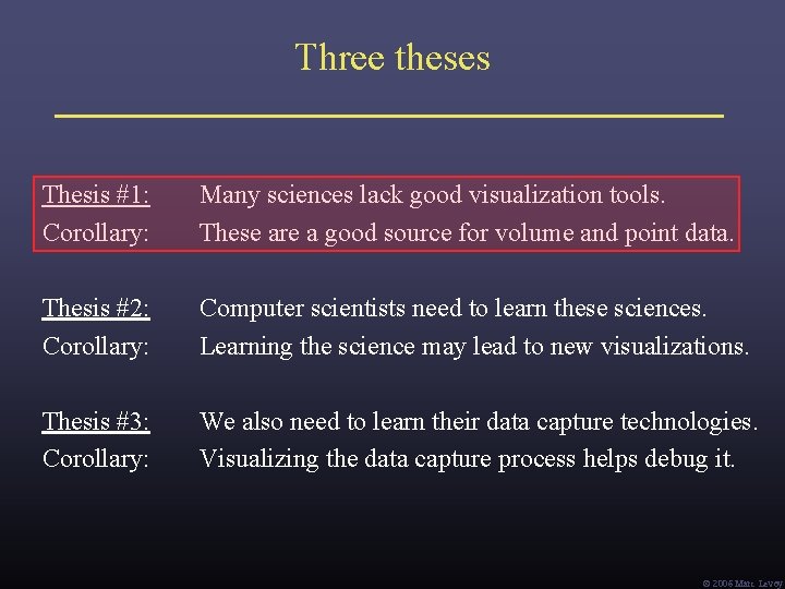
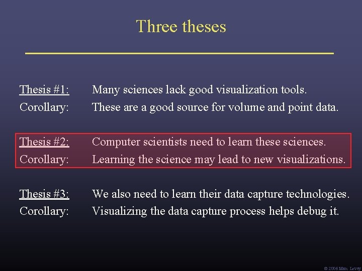
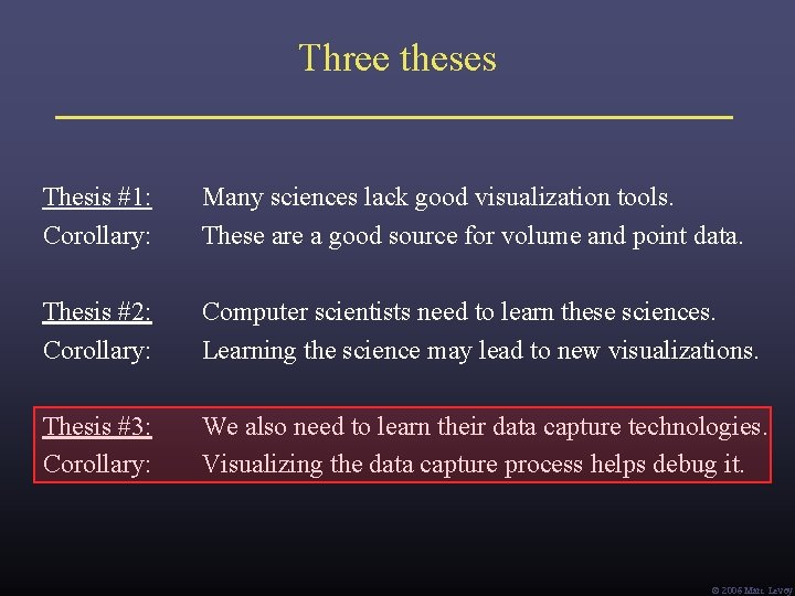
Three theses Thesis #1: Corollary: Many sciences lack good visualization tools. These are a good source for volume and point data. Thesis #2: Corollary: Computer scientists need to learn these sciences. Learning the science may lead to new visualizations. Thesis #3: Corollary: We also need to learn their data capture technologies. Visualizing the data capture process helps debug it. Ó 2006 Marc Levoy

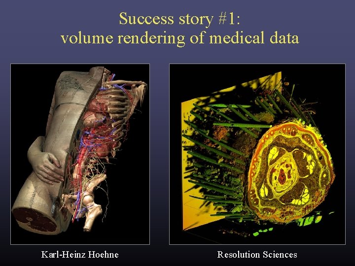
Success story #1: volume rendering of medical data Karl-Heinz Hoehne Resolution Sciences

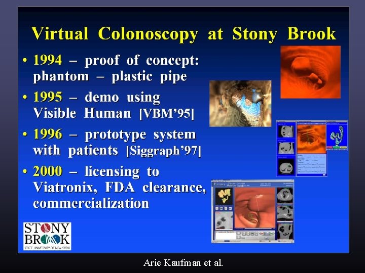
Success story #1: volume rendering of medical data Arie Kaufman et al.

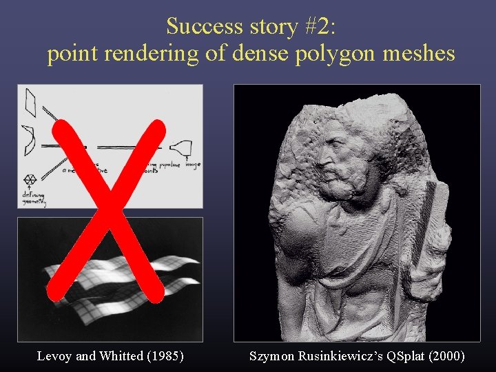
Success story #2: point rendering of dense polygon meshes Levoy and Whitted (1985) Szymon Rusinkiewicz’s QSplat (2000)

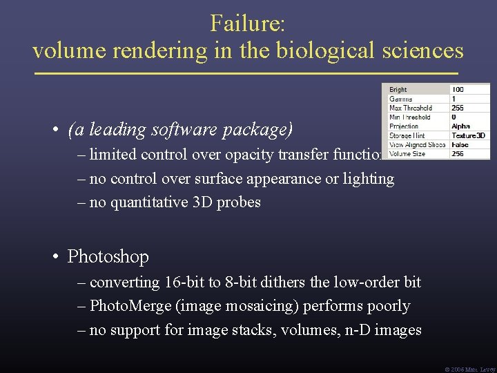
Failure: volume rendering in the biological sciences • (a leading software package) – limited control over opacity transfer function – no control over surface appearance or lighting – no quantitative 3 D probes • Photoshop – converting 16 -bit to 8 -bit dithers the low-order bit – Photo. Merge (image mosaicing) performs poorly – no support for image stacks, volumes, n-D images Ó 2006 Marc Levoy

What’s going on in the basic sciences? • new instruments scientific discoveries • most important new instrument in the last 50 years: the digital computer • computers + digital sensors = computational imaging Def: imaging methods in which computation is inherent in image formation. – B. K. Horn • the revolution in medical imaging (CT, MR, PET, etc. ) is now happening all across the basic sciences (It’s also a great source for volume and point data!) Ó 2006 Marc Levoy

Examples of computational imaging in the sciences • medical imaging – rebinning inspiration for light field rendering ü – transmission tomography – reflection tomography (for ultrasound) • geophysics ü – borehole tomography – seismic reflection surveying • applied physics ü – diffuse optical tomography ü – diffraction tomography ü in this talk ü – scattering and inverse scattering Ó 2006 Marc Levoy

• biology ü – confocal microscopy applicable at macro scale too ü – deconvolution microscopy • astronomy ü – coded-aperture imaging – interferometric imaging • airborne sensing – multi-perspective panoramas – synthetic aperture radar Ó 2006 Marc Levoy

• optics – holography – wavefront coding Ó 2006 Marc Levoy

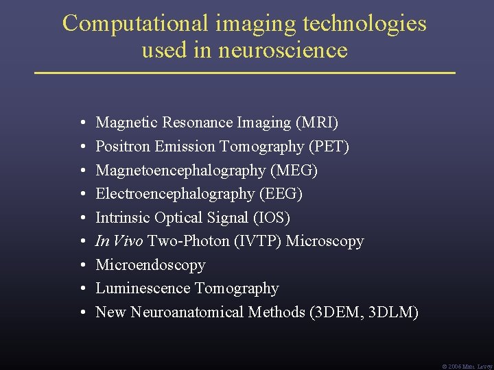
Computational imaging technologies used in neuroscience • • • Magnetic Resonance Imaging (MRI) Positron Emission Tomography (PET) Magnetoencephalography (MEG) Electroencephalography (EEG) Intrinsic Optical Signal (IOS) In Vivo Two-Photon (IVTP) Microscopy Microendoscopy Luminescence Tomography New Neuroanatomical Methods (3 DEM, 3 DLM) Ó 2006 Marc Levoy

The Fourier projection-slice theorem (a. k. a. the central section theorem) [Bracewell 1956] P (t ) G (ω) (from Kak) • • P (t) is the integral of g(x, y) in the direction G(u, v) is the 2 D Fourier transform of g(x, y) G (ω) is a 1 D slice of this transform taken at -1 { G (ω) } = P (t) ! Ó 2006 Marc Levoy

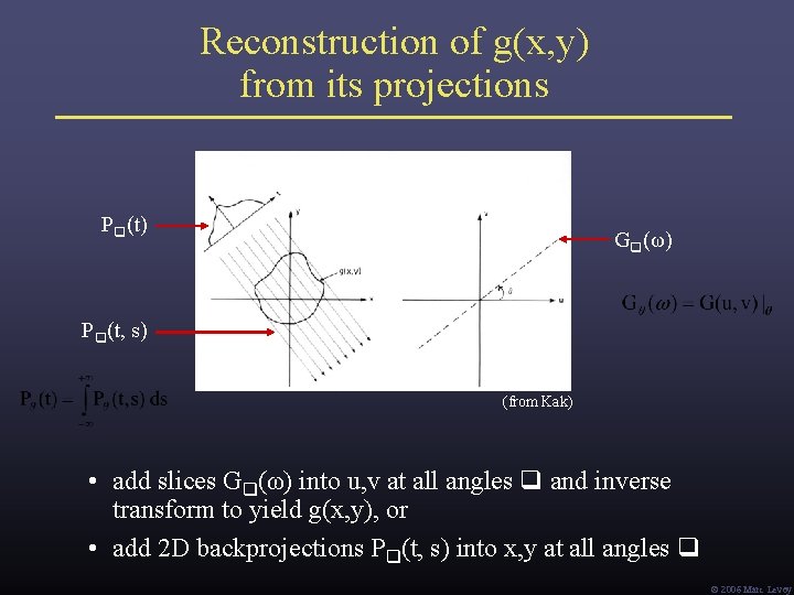
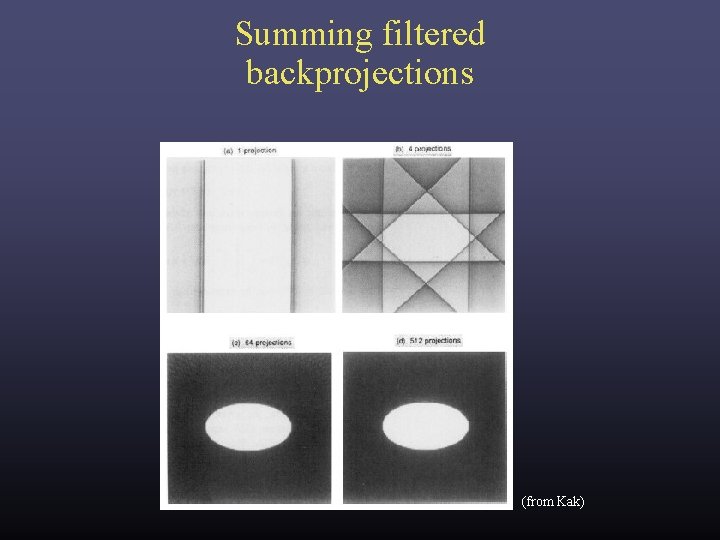
Reconstruction of g(x, y) from its projections P (t) G (ω) P (t, s) (from Kak) • add slices G (ω) into u, v at all angles and inverse transform to yield g(x, y), or • add 2 D backprojections P (t, s) into x, y at all angles Ó 2006 Marc Levoy

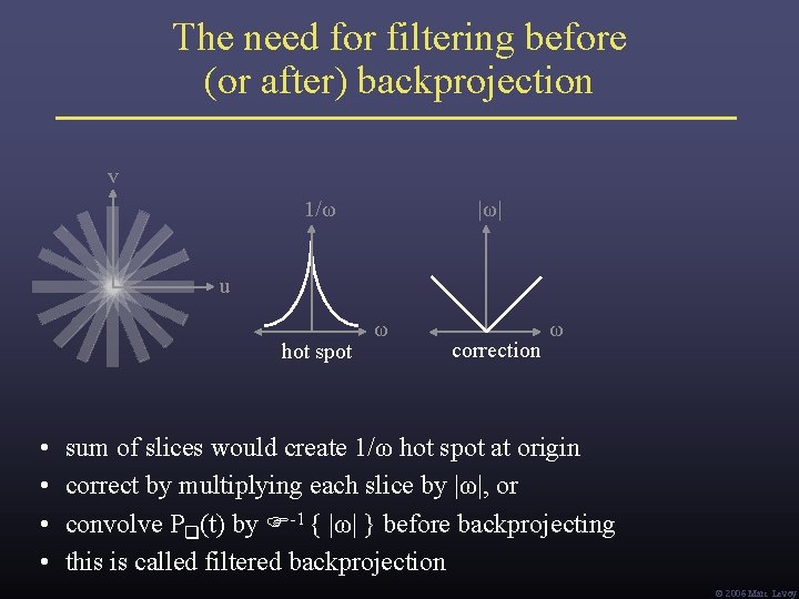
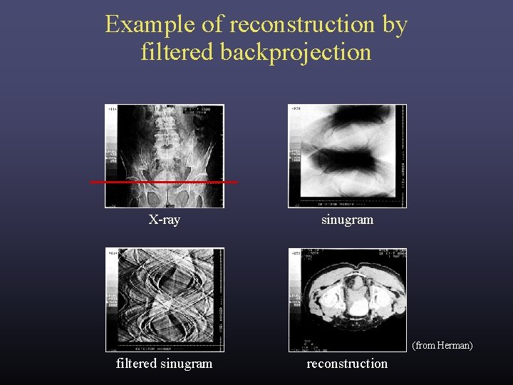
The need for filtering before (or after) backprojection v 1/ω |ω| u hot spot • • ω correction ω sum of slices would create 1/ω hot spot at origin correct by multiplying each slice by |ω|, or convolve P (t) by -1 { |ω| } before backprojecting this is called filtered backprojection Ó 2006 Marc Levoy

Summing filtered backprojections (from Kak)

Example of reconstruction by filtered backprojection X-ray sinugram (from Herman) filtered sinugram reconstruction

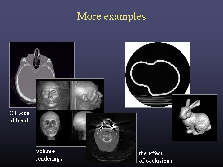
More examples CT scan of head volume renderings the effect of occlusions

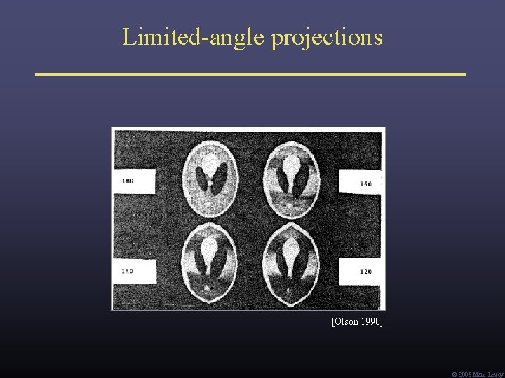
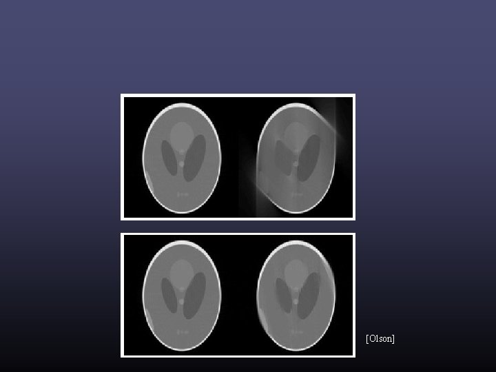
Limited-angle projections [Olson 1990] Ó 2006 Marc Levoy

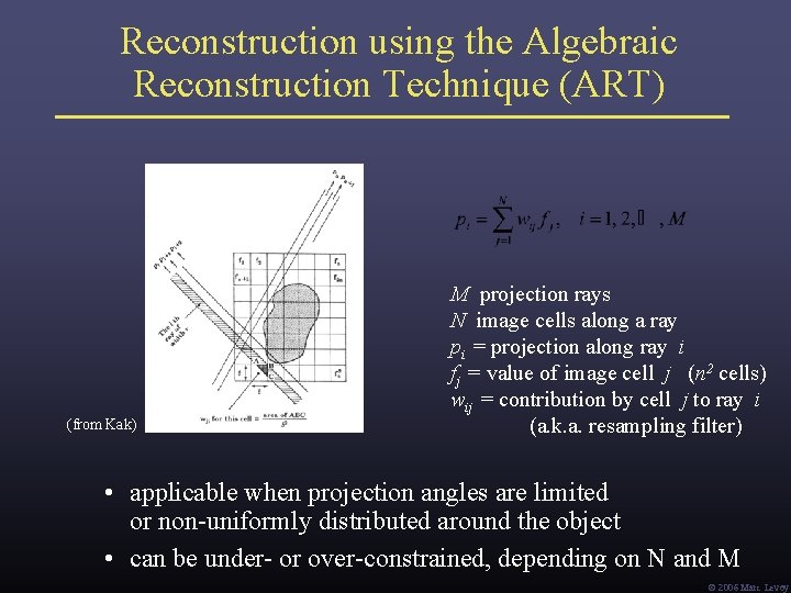
Reconstruction using the Algebraic Reconstruction Technique (ART) (from Kak) M projection rays N image cells along a ray pi = projection along ray i fj = value of image cell j (n 2 cells) wij = contribution by cell j to ray i (a. k. a. resampling filter) • applicable when projection angles are limited or non-uniformly distributed around the object • can be under- or over-constrained, depending on N and M Ó 2006 Marc Levoy

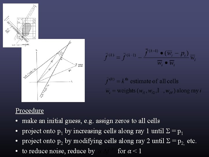
Procedure • make an initial guess, e. g. assign zeros to all cells • project onto p 1 by increasing cells along ray 1 until Σ = p 1 • project onto p 2 by modifying cells along ray 2 until Σ = p 2, etc. • to reduce noise, reduce by for α < 1

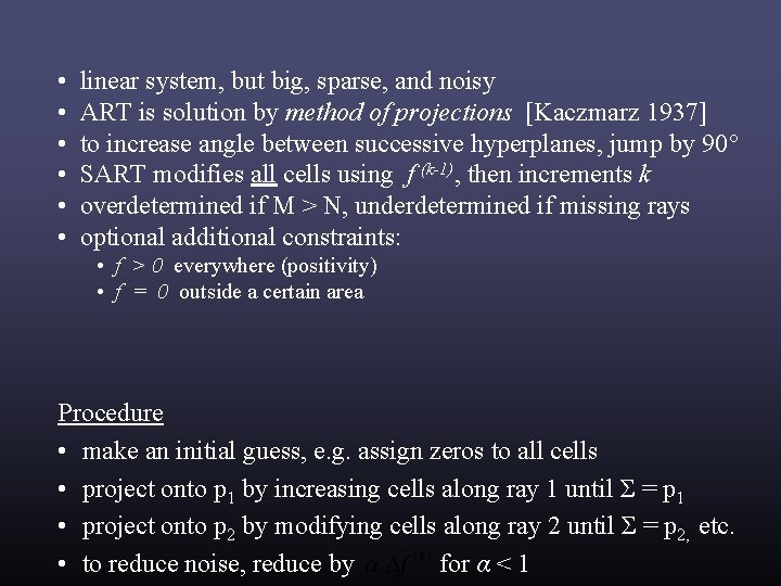
• • • linear system, but big, sparse, and noisy ART is solution by method of projections [Kaczmarz 1937] to increase angle between successive hyperplanes, jump by 90° SART modifies all cells using f (k-1), then increments k overdetermined if M > N, underdetermined if missing rays optional additional constraints: • f > 0 everywhere (positivity) • f = 0 outside a certain area Procedure • make an initial guess, e. g. assign zeros to all cells • project onto p 1 by increasing cells along ray 1 until Σ = p 1 • project onto p 2 by modifying cells along ray 2 until Σ = p 2, etc. • to reduce noise, reduce by for α < 1

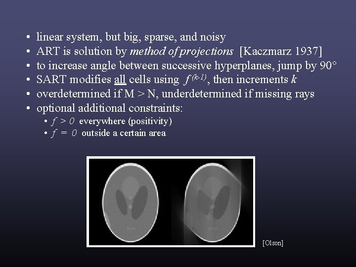
• • • linear system, but big, sparse, and noisy ART is solution by method of projections [Kaczmarz 1937] to increase angle between successive hyperplanes, jump by 90° SART modifies all cells using f (k-1), then increments k overdetermined if M > N, underdetermined if missing rays optional additional constraints: • f > 0 everywhere (positivity) • f = 0 outside a certain area [Olson]

[Olson]

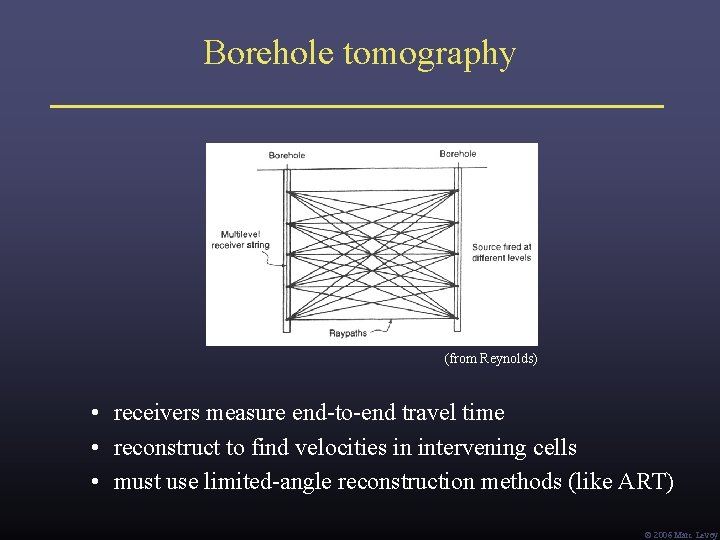
Borehole tomography (from Reynolds) • receivers measure end-to-end travel time • reconstruct to find velocities in intervening cells • must use limited-angle reconstruction methods (like ART) Ó 2006 Marc Levoy

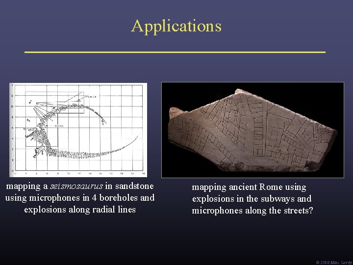
Applications mapping a seismosaurus in sandstone using microphones in 4 boreholes and explosions along radial lines mapping ancient Rome using explosions in the subways and microphones along the streets? Ó 2006 Marc Levoy

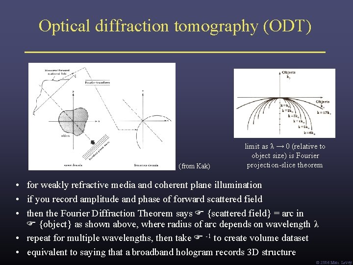
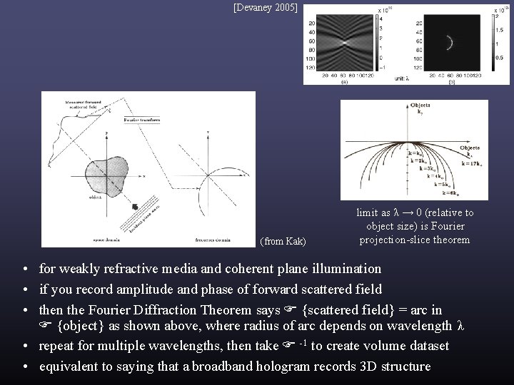
Optical diffraction tomography (ODT) (from Kak) limit as λ → 0 (relative to object size) is Fourier projection-slice theorem • for weakly refractive media and coherent plane illumination • if you record amplitude and phase of forward scattered field • then the Fourier Diffraction Theorem says {scattered field} = arc in {object} as shown above, where radius of arc depends on wavelength λ • repeat for multiple wavelengths, then take -1 to create volume dataset • equivalent to saying that a broadband hologram records 3 D structure Ó 2006 Marc Levoy

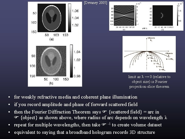
[Devaney 2005] (from Kak) limit as λ → 0 (relative to object size) is Fourier projection-slice theorem • for weakly refractive media and coherent plane illumination • if you record amplitude and phase of forward scattered field • then the Fourier Diffraction Theorem says {scattered field} = arc in {object} as shown above, where radius of arc depends on wavelength λ • repeat for multiple wavelengths, then take -1 to create volume dataset • equivalent to saying that a broadband hologram records 3 D structure

[Devaney 2005] limit as λ → 0 (relative to object size) is Fourier projection-slice theorem • for weakly refractive media and coherent plane illumination • if you record amplitude and phase of forward scattered field • then the Fourier Diffraction Theorem says {scattered field} = arc in {object} as shown above, where radius of arc depends on wavelength λ • repeat for multiple wavelengths, then take -1 to create volume dataset • equivalent to saying that a broadband hologram records 3 D structure

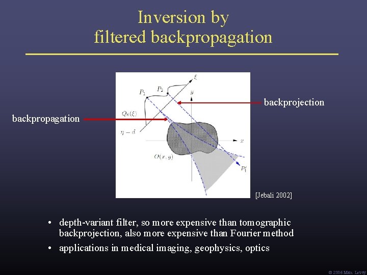
Inversion by filtered backpropagation backprojection backpropagation [Jebali 2002] • depth-variant filter, so more expensive than tomographic backprojection, also more expensive than Fourier method • applications in medical imaging, geophysics, optics Ó 2006 Marc Levoy

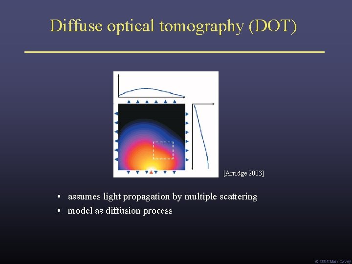
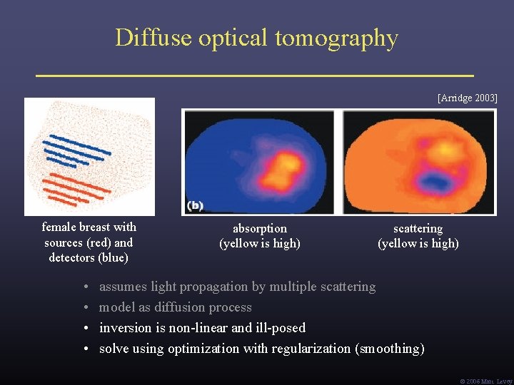
Diffuse optical tomography (DOT) [Arridge 2003] • assumes light propagation by multiple scattering • model as diffusion process Ó 2006 Marc Levoy

Diffuse optical tomography [Arridge 2003] female breast with sources (red) and detectors (blue) • • absorption (yellow is high) scattering (yellow is high) assumes light propagation by multiple scattering model as diffusion process inversion is non-linear and ill-posed solve using optimization with regularization (smoothing) Ó 2006 Marc Levoy

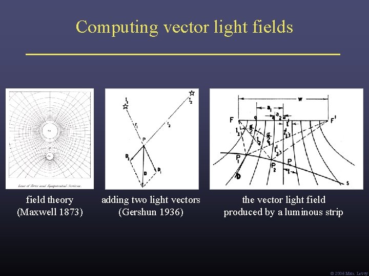
Computing vector light fields field theory (Maxwell 1873) adding two light vectors (Gershun 1936) the vector light field produced by a luminous strip Ó 2006 Marc Levoy

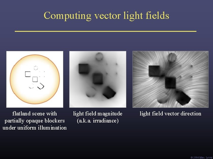
Computing vector light fields flatland scene with partially opaque blockers under uniform illumination light field magnitude (a. k. a. irradiance) light field vector direction Ó 2006 Marc Levoy

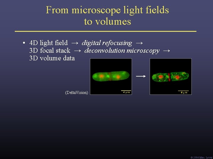
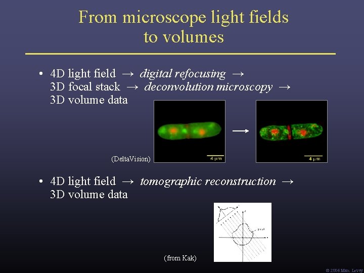
From microscope light fields to volumes • 4 D light field → digital refocusing → 3 D focal stack → deconvolution microscopy → 3 D volume data (Delta. Vision) Ó 2006 Marc Levoy

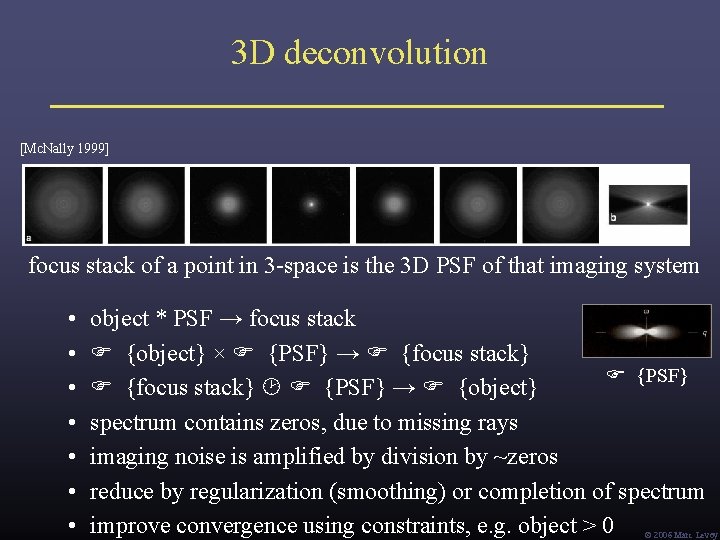
3 D deconvolution [Mc. Nally 1999] focus stack of a point in 3 -space is the 3 D PSF of that imaging system • • object * PSF → focus stack {object} × {PSF} → {focus stack} {PSF} {focus stack} {PSF} → {object} spectrum contains zeros, due to missing rays imaging noise is amplified by division by ~zeros reduce by regularization (smoothing) or completion of spectrum improve convergence using constraints, e. g. object > 0 Ó 2006 Marc Levoy

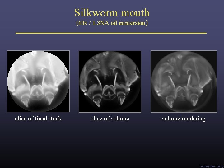
Silkworm mouth (40 x / 1. 3 NA oil immersion) slice of focal stack slice of volume rendering Ó 2006 Marc Levoy

From microscope light fields to volumes • 4 D light field → digital refocusing → 3 D focal stack → deconvolution microscopy → 3 D volume data (Delta. Vision) • 4 D light field → tomographic reconstruction → 3 D volume data (from Kak) Ó 2006 Marc Levoy

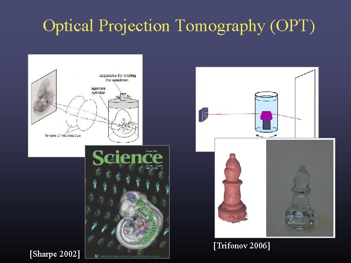
Optical Projection Tomography (OPT) [Sharpe 2002] [Trifonov 2006]

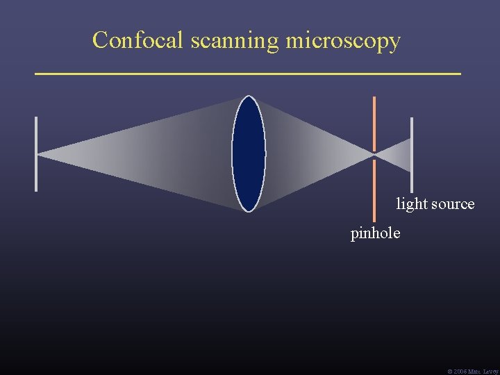
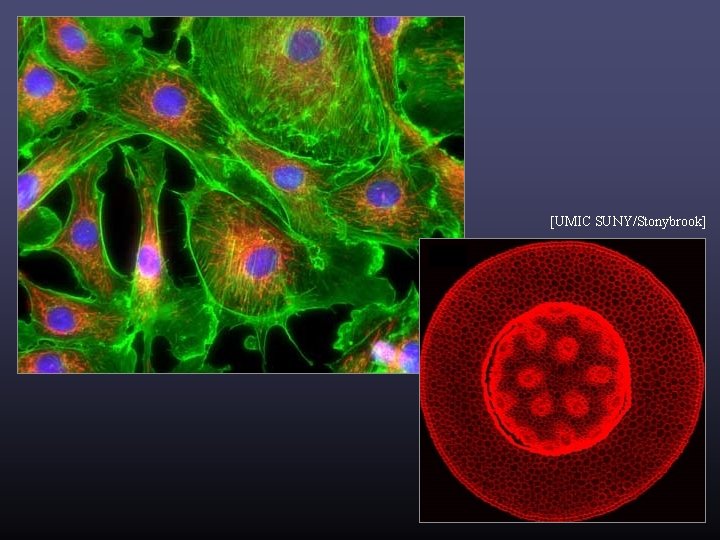
Confocal scanning microscopy light source pinhole Ó 2006 Marc Levoy

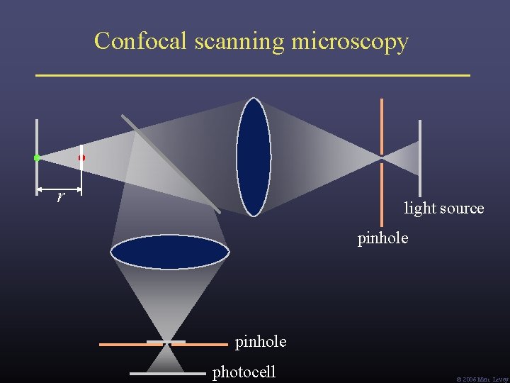
Confocal scanning microscopy r light source pinhole photocell Ó 2006 Marc Levoy

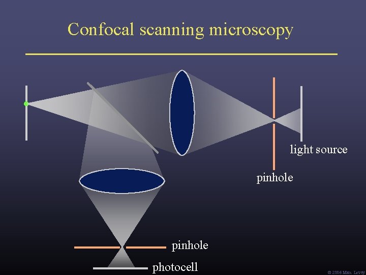
Confocal scanning microscopy light source pinhole photocell Ó 2006 Marc Levoy

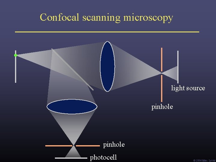
Confocal scanning microscopy light source pinhole photocell Ó 2006 Marc Levoy

[UMIC SUNY/Stonybrook]

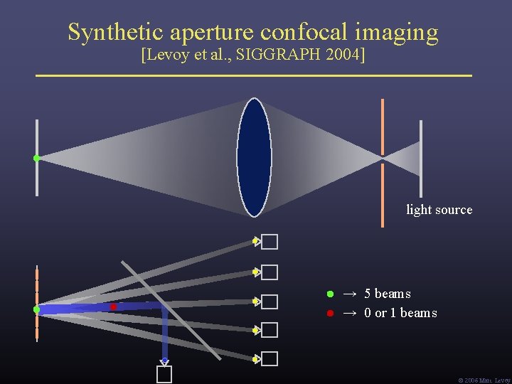
Synthetic aperture confocal imaging [Levoy et al. , SIGGRAPH 2004] light source → 5 beams → 0 or 1 beams Ó 2006 Marc Levoy

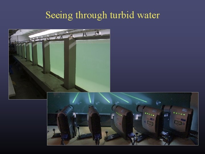
Seeing through turbid water

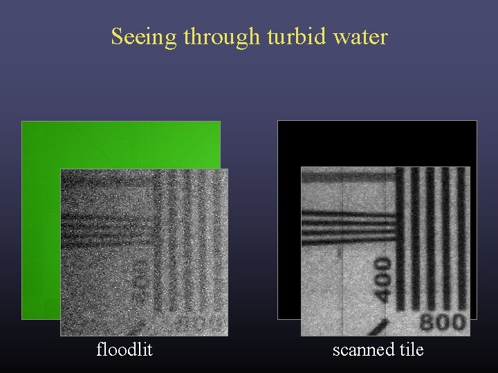
Seeing through turbid water floodlit scanned tile

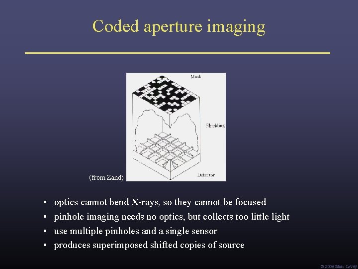
Coded aperture imaging (from Zand) • • optics cannot bend X-rays, so they cannot be focused pinhole imaging needs no optics, but collects too little light use multiple pinholes and a single sensor produces superimposed shifted copies of source Ó 2006 Marc Levoy

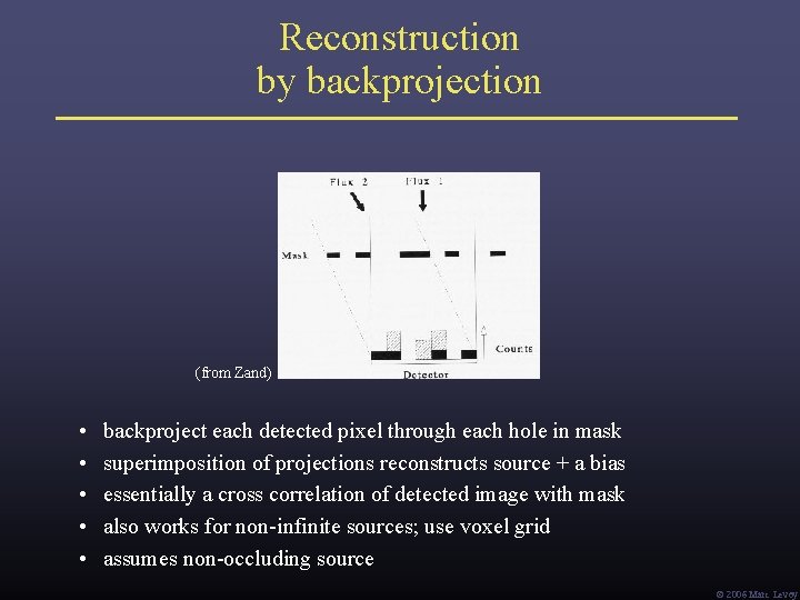
Reconstruction by backprojection (from Zand) • • • backproject each detected pixel through each hole in mask superimposition of projections reconstructs source + a bias essentially a cross correlation of detected image with mask also works for non-infinite sources; use voxel grid assumes non-occluding source Ó 2006 Marc Levoy

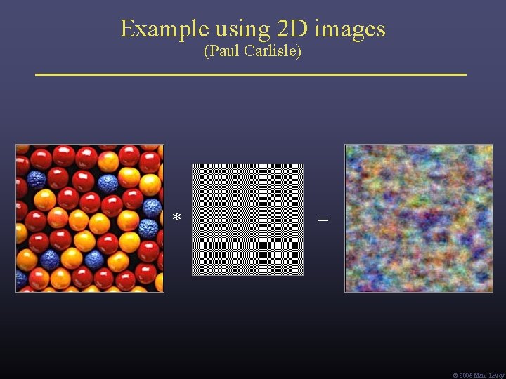
Example using 2 D images (Paul Carlisle) * = Ó 2006 Marc Levoy

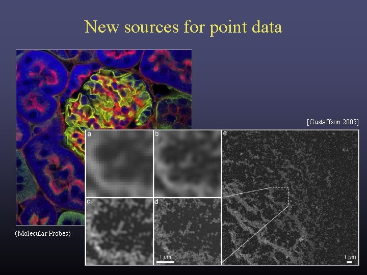
New sources for point data [Gustaffson 2005] (Molecular Probes)

Three theses Thesis #1: Corollary: Many sciences lack good visualization tools. These are a good source for volume and point data. Thesis #2: Corollary: Computer scientists need to learn these sciences. Learning the science may lead to new visualizations. Thesis #3: Corollary: We also need to learn their data capture technologies. Visualizing the data capture process helps debug it. Ó 2006 Marc Levoy

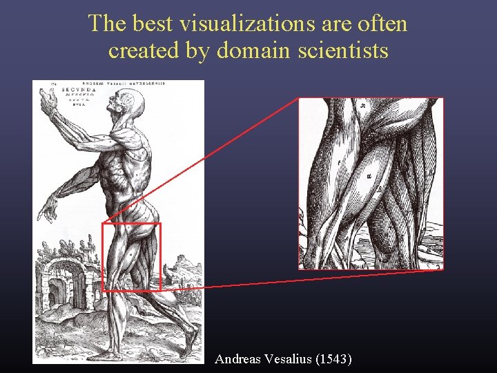
The best visualizations are often created by domain scientists Andreas Vesalius (1543)

Three theses Thesis #1: Corollary: Many sciences lack good visualization tools. These are a good source for volume and point data. Thesis #2: Corollary: Computer scientists need to learn these sciences. Learning the science may lead to new visualizations. Thesis #3: Corollary: We also need to learn their data capture technologies. Visualizing the data capture process helps debug it. Ó 2006 Marc Levoy

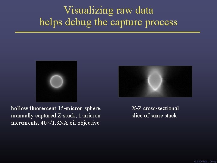
Visualizing raw data helps debug the capture process hollow fluorescent 15 -micron sphere, manually captured Z-stack, 1 -micron increments, 40×/1. 3 NA oil objective X-Z cross-sectional slice of same stack Ó 2006 Marc Levoy

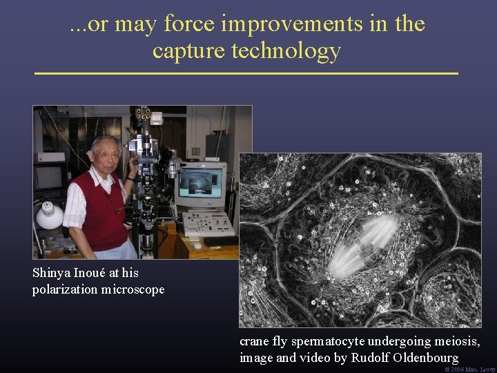
. . . or may force improvements in the capture technology Shinya Inoué at his polarization microscope crane fly spermatocyte undergoing meiosis, image and video by Rudolf Oldenbourg Ó 2006 Marc Levoy

Final thought: the importance of building useful tools “A toolmaker succeeds as, and only as, the users of his tool succeed with his aid. However shining the blade, however jeweled the hilt, however perfect the heft, a sword is tested only by cutting. That swordsmith is successful whose clients die of old age. ” – Fred Brooks, Computer Scientist as Toolsmith – II, Proc. CACM 1996 Ó 2006 Marc Levoy

Acknowledgements • • Fred Brooks (“Computer Scientist as Toolsmith”) Pat Hanrahan (“Self-Illustrating Phenomena”) Bill Lorensen (“The Death of Visualization”) Shinya Inoué (“History of Polarization Microscopy”) Ó 2006 Marc Levoy