Where did the variogram come from Geology Biology

Where did the variogram come from? Geology? Biology? Oceanography? Physics?

Actually, some of the earliest references were from 1926. A Swedish forester, A. Langsaeter, used this method to express variation when dealing with systematic sampling in forest surveys.

A plea for exploratory data analysis… We shall not cease from exploration And the end of all our exploring Will be to arrive where we started And know the place for the first time. (T. S. Eliot)

Quantifying scale of variation with semivariograms What is spatial dependence, autocorrelation? • Euclidean vs. network distance • Geographical Information System (GIS) ? (Ganio, Torgersen, and Gresswell 2005, Frontiers in Ecology and the Environment)

Distribution and abundance Age 1+ coastal cutthroat trout 0 1 km (Gresswell, Torgersen, and Bateman 2006, Influence of landscape on stream habitats and biological assemblages)

Fine- and coarsescale patterns Pool Riffle/rapid Cascade 12 9 7 3 0 (Torgersen et al. 2004, GIS in Fisheries and Aquatic Sciences) 350 m

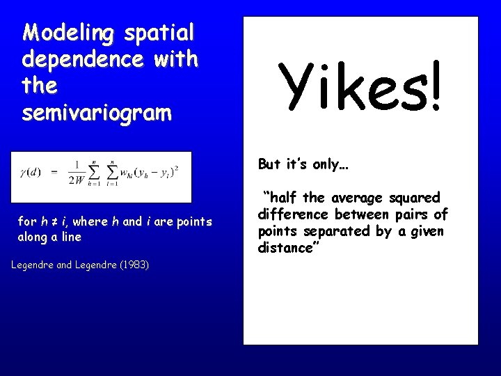
Modeling spatial dependence with the semivariogram Yikes! But it’s only… for h ≠ i, where h and i are points along a line Legendre and Legendre (1983) “half the average squared difference between pairs of points separated by a given distance”

Modeling spatial dependence with the semivariogram for h ≠ i, where h and i are points along a line Legendre and Legendre (1983) A simple example… Point. ID x-coord y A 1 1 6 B 2 1 8 C 3 1 9 D 5 1 7 E 8 1 16 F 9 1 14 G 11 1 11 H 12 1 9

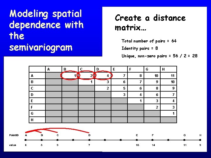
Modeling spatial dependence with the semivariogram A A B C D E F G H B Create a distance matrix… Total number of pairs = 64 Identity pairs = 8 Unique, non-zero pairs = 56 / 2 = 28 C 1 D E F G H 2 4 7 8 10 11 1 3 6 7 9 10 2 5 6 8 9 3 4 6 7 1 3 4 2 3 1

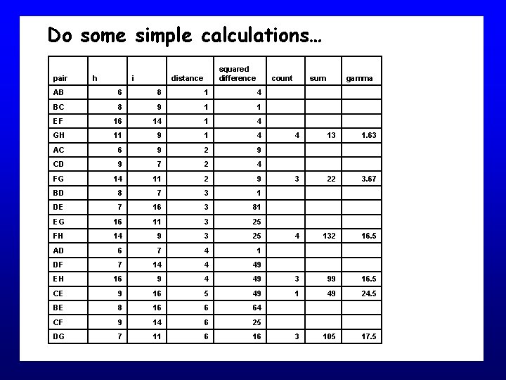
Do some simple calculations… pair h i squared difference distance count AB 6 8 1 4 BC 8 9 1 1 EF 16 14 1 4 GH 11 9 1 4 AC 6 9 2 9 CD 9 7 2 4 FG 14 11 2 9 BD 8 7 3 1 DE 7 16 3 81 EG 16 11 3 25 FH 14 9 3 25 AD 6 7 4 1 DF 7 14 4 49 EH 16 9 4 CE 9 16 BE 8 CF DG sum gamma 4 13 1. 63 3 22 3. 67 4 132 16. 5 49 3 99 16. 5 5 49 1 49 24. 5 16 6 64 9 14 6 25 7 11 6 16 3 105 17. 5

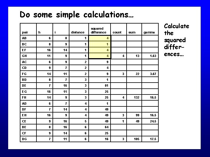
Do some simple calculations… pair h i squared difference distance count AB 6 8 1 4 BC 8 9 1 1 EF 16 14 1 4 GH 11 9 1 4 AC 6 9 2 9 CD 9 7 2 4 FG 14 11 2 9 BD 8 7 3 1 DE 7 16 3 81 EG 16 11 3 25 FH 14 9 3 25 AD 6 7 4 1 DF 7 14 4 49 EH 16 9 4 CE 9 16 BE 8 CF DG sum gamma 4 13 1. 63 3 22 3. 67 4 132 16. 5 49 3 99 16. 5 5 49 1 49 24. 5 16 6 64 9 14 6 25 7 11 6 16 3 105 17. 5 Calculate the squared differences…

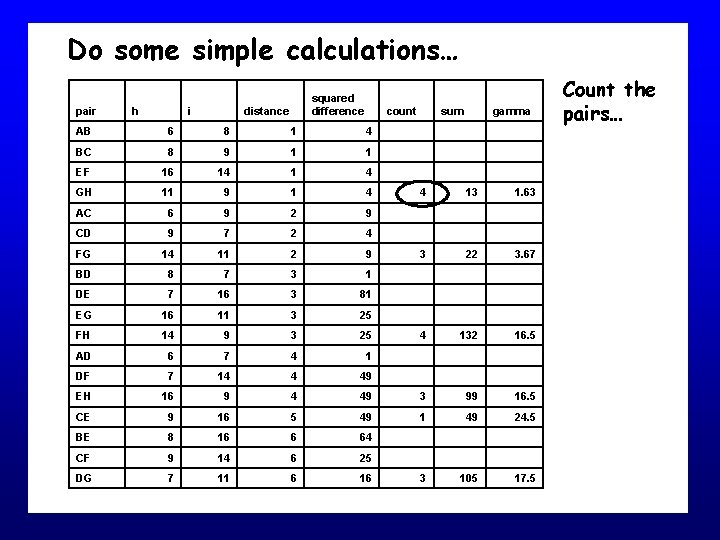
Do some simple calculations… pair h i squared difference distance count AB 6 8 1 4 BC 8 9 1 1 EF 16 14 1 4 GH 11 9 1 4 AC 6 9 2 9 CD 9 7 2 4 FG 14 11 2 9 BD 8 7 3 1 DE 7 16 3 81 EG 16 11 3 25 FH 14 9 3 25 AD 6 7 4 1 DF 7 14 4 49 EH 16 9 4 CE 9 16 BE 8 CF DG sum gamma 4 13 1. 63 3 22 3. 67 4 132 16. 5 49 3 99 16. 5 5 49 1 49 24. 5 16 6 64 9 14 6 25 7 11 6 16 3 105 17. 5 Count the pairs…

Do some simple calculations… pair h i squared difference distance count AB 6 8 1 4 BC 8 9 1 1 EF 16 14 1 4 GH 11 9 1 4 AC 6 9 2 9 CD 9 7 2 4 FG 14 11 2 9 BD 8 7 3 1 DE 7 16 3 81 EG 16 11 3 25 FH 14 9 3 25 AD 6 7 4 1 DF 7 14 4 49 EH 16 9 4 CE 9 16 BE 8 CF DG sum gamma 4 13 1. 63 3 22 3. 67 4 132 16. 5 49 3 99 16. 5 5 49 1 49 24. 5 16 6 64 9 14 6 25 7 11 6 16 3 105 17. 5 Sum the squared differences…

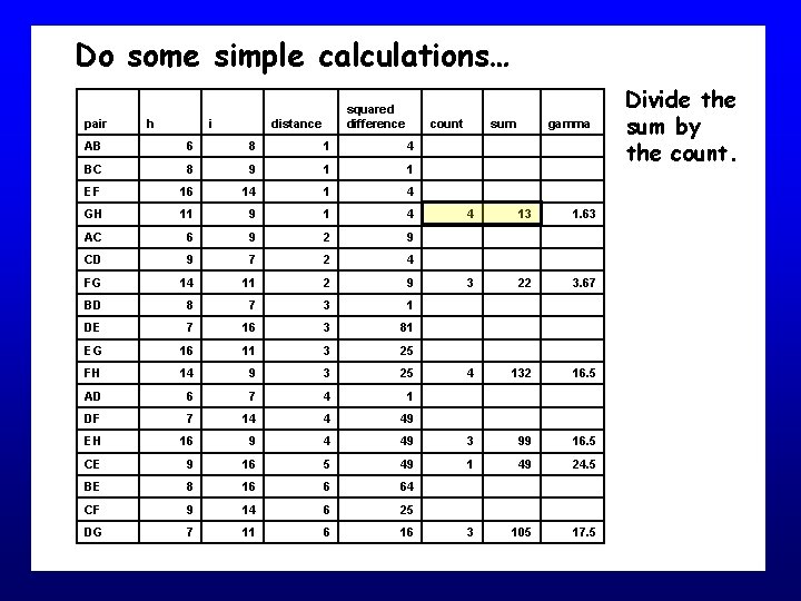
Do some simple calculations… pair h i squared difference distance count AB 6 8 1 4 BC 8 9 1 1 EF 16 14 1 4 GH 11 9 1 4 AC 6 9 2 9 CD 9 7 2 4 FG 14 11 2 9 BD 8 7 3 1 DE 7 16 3 81 EG 16 11 3 25 FH 14 9 3 25 AD 6 7 4 1 DF 7 14 4 49 EH 16 9 4 CE 9 16 BE 8 CF DG sum gamma 4 13 1. 63 3 22 3. 67 4 132 16. 5 49 3 99 16. 5 5 49 1 49 24. 5 16 6 64 9 14 6 25 7 11 6 16 3 105 17. 5 Divide the sum by the count.

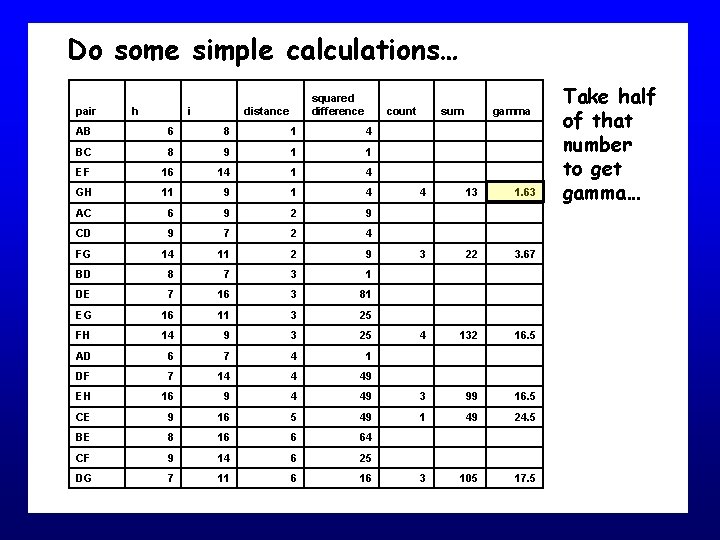
Do some simple calculations… pair h i squared difference distance count AB 6 8 1 4 BC 8 9 1 1 EF 16 14 1 4 GH 11 9 1 4 AC 6 9 2 9 CD 9 7 2 4 FG 14 11 2 9 BD 8 7 3 1 DE 7 16 3 81 EG 16 11 3 25 FH 14 9 3 25 AD 6 7 4 1 DF 7 14 4 49 EH 16 9 4 CE 9 16 BE 8 CF DG sum gamma 4 13 1. 63 3 22 3. 67 4 132 16. 5 49 3 99 16. 5 5 49 1 49 24. 5 16 6 64 9 14 6 25 7 11 6 16 3 105 17. 5 Take half of that number to get gamma…

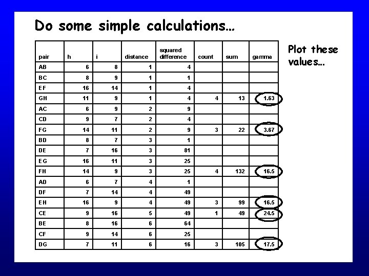
Do some simple calculations… pair h i squared difference distance count AB 6 8 1 4 BC 8 9 1 1 EF 16 14 1 4 GH 11 9 1 4 AC 6 9 2 9 CD 9 7 2 4 FG 14 11 2 9 BD 8 7 3 1 DE 7 16 3 81 EG 16 11 3 25 FH 14 9 3 25 AD 6 7 4 1 DF 7 14 4 49 EH 16 9 4 CE 9 16 BE 8 CF DG sum gamma 4 13 1. 63 3 22 3. 67 4 132 16. 5 49 3 99 16. 5 5 49 1 49 24. 5 16 6 64 9 14 6 25 7 11 6 16 3 105 17. 5 Plot these values…

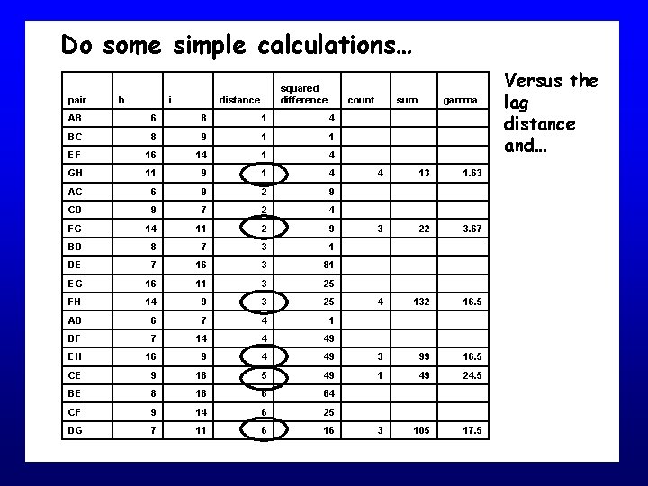
Do some simple calculations… pair h i squared difference distance count AB 6 8 1 4 BC 8 9 1 1 EF 16 14 1 4 GH 11 9 1 4 AC 6 9 2 9 CD 9 7 2 4 FG 14 11 2 9 BD 8 7 3 1 DE 7 16 3 81 EG 16 11 3 25 FH 14 9 3 25 AD 6 7 4 1 DF 7 14 4 49 EH 16 9 4 CE 9 16 BE 8 CF DG sum gamma 4 13 1. 63 3 22 3. 67 4 132 16. 5 49 3 99 16. 5 5 49 1 49 24. 5 16 6 64 9 14 6 25 7 11 6 16 3 105 17. 5 Versus the lag distance and…

Voilà, the semivariogram!

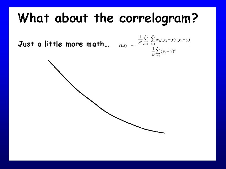
What about the correlogram? Just a little more math…

Semivariance Anatomy of the semivariogram Slope Nugget Range Separation distance Sill

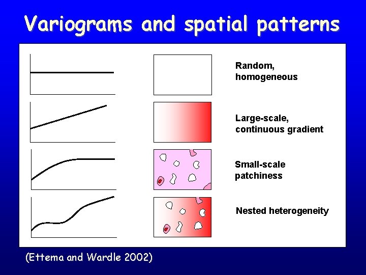
Variograms and spatial patterns Random, homogeneous Large-scale, continuous gradient Small-scale patchiness Nested heterogeneity (Ettema and Wardle 2002)

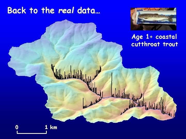
Back to the real data… Age 1+ coastal cutthroat trout 0 1 km

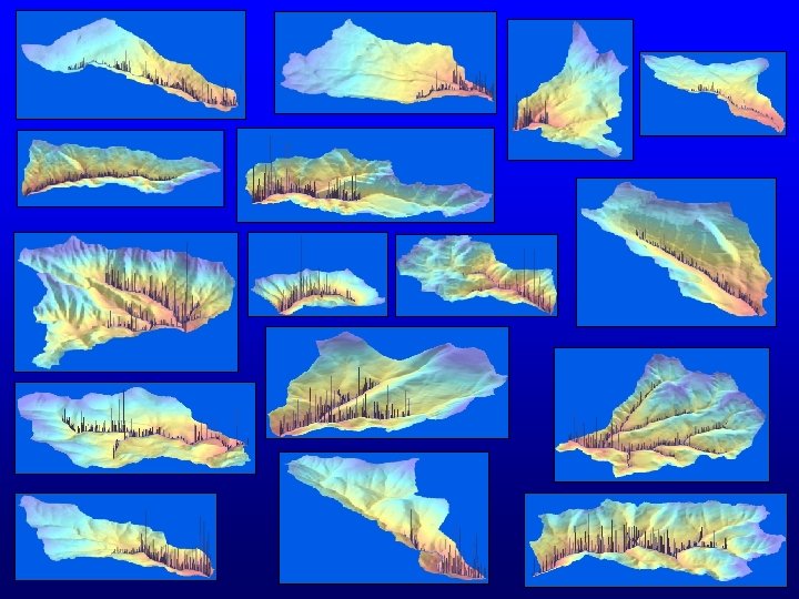
Network variogram of fish counts… Semivariogram • Fitted spherical model Randomization • Test of spatial dependence (Torgersen et al. 2004)

(Ganio et al. 2005)

(Ganio et al. 2005)

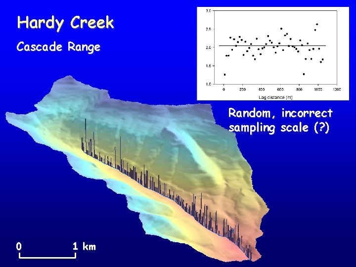
Hardy Creek Cascade Range Random, incorrect sampling scale (? ) 0 1 km

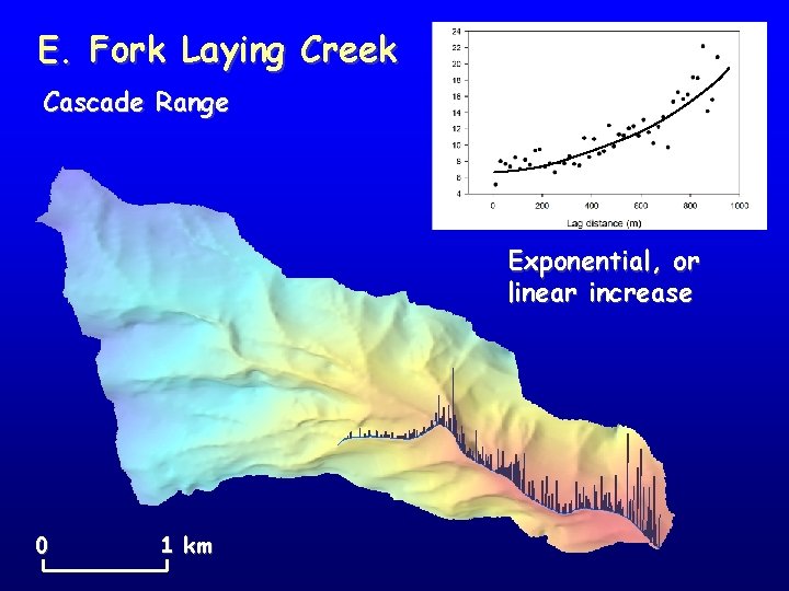
E. Fork Laying Creek Cascade Range Exponential, or linear increase 0 1 km

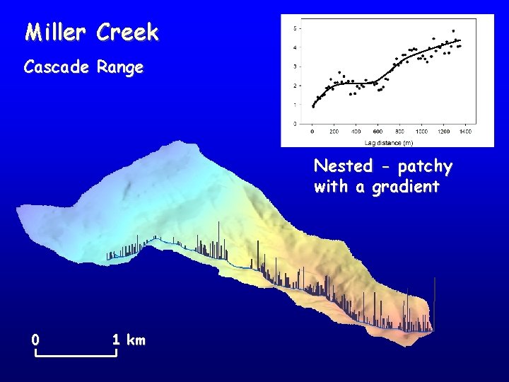
Miller Creek Cascade Range Nested - patchy with a gradient 0 1 km

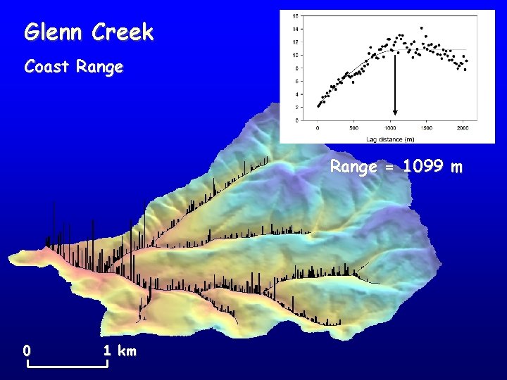
Glenn Creek Coast Range = 1099 m 0 1 km

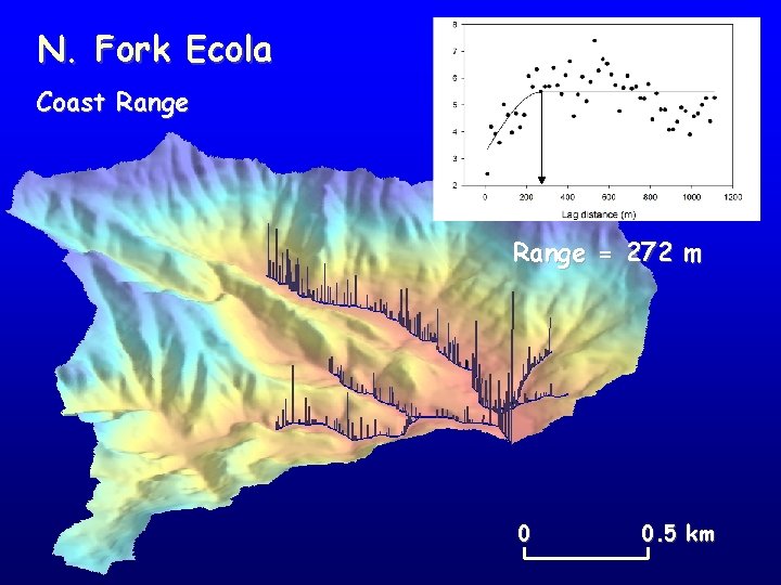
N. Fork Ecola Coast Range = 272 m 0 0. 5 km

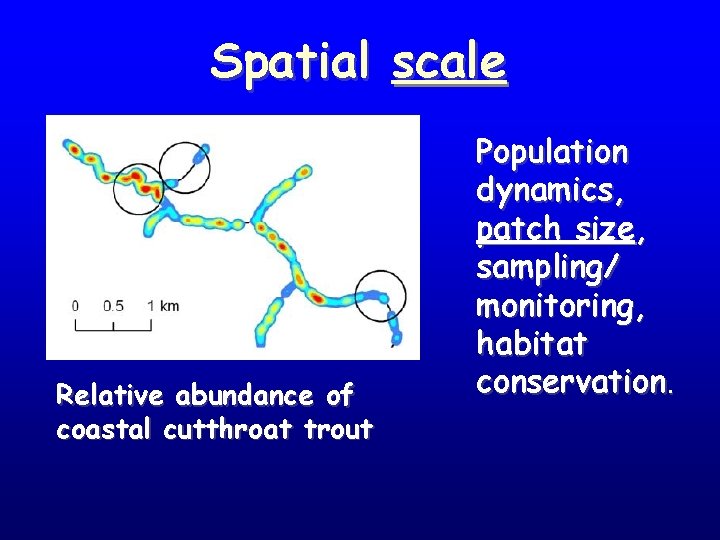
Spatial scale Relative abundance of coastal cutthroat trout Population dynamics, patch size, sampling/ monitoring, habitat conservation.

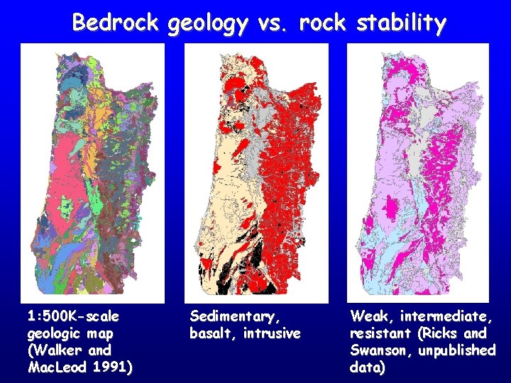
Bedrock geology vs. rock stability 1: 500 K-scale geologic map (Walker and Mac. Leod 1991) Sedimentary, basalt, intrusive Weak, intermediate, resistant (Ricks and Swanson, unpublished data)

Spatial variability in fish distribution and landscape characteristics Range is often interpreted as the average patch size.

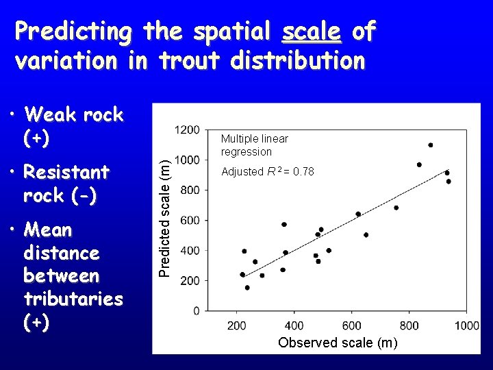
Predicting the spatial scale of variation in trout distribution • Weak rock (+) • Mean distance between tributaries (+) Predicted scale (m) • Resistant rock (-) Multiple linear regression Adjusted R 2 = 0. 78 Observed scale (m)

Conclusions • Coastal cutthroat trout distribution exhibited strong spatial structuring at scales of 200 -1000 m. • Empirical variograms provided an effective means to compare spatial structure among watersheds. • Scale of variation (patch size) in trout distribution corresponded with landscape characteristics.

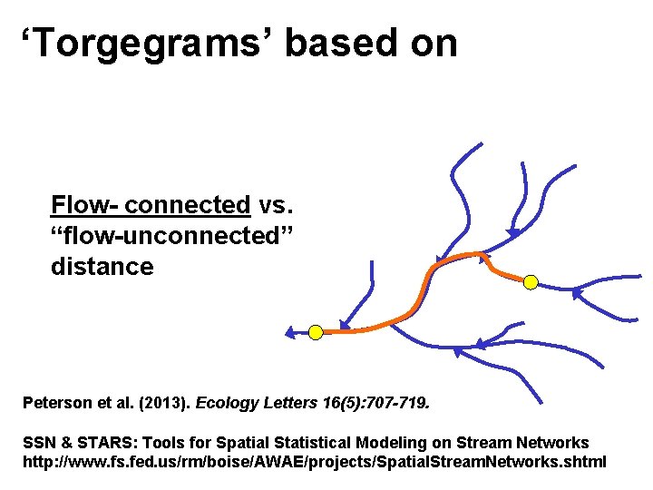
‘Torgegrams’ based on Flow- connected vs. “flow-unconnected” distance ? Peterson et al. (2013). Ecology Letters 16(5): 707 -719. SSN & STARS: Tools for Spatial Statistical Modeling on Stream Networks http: //www. fs. fed. us/rm/boise/AWAE/projects/Spatial. Stream. Networks. shtml

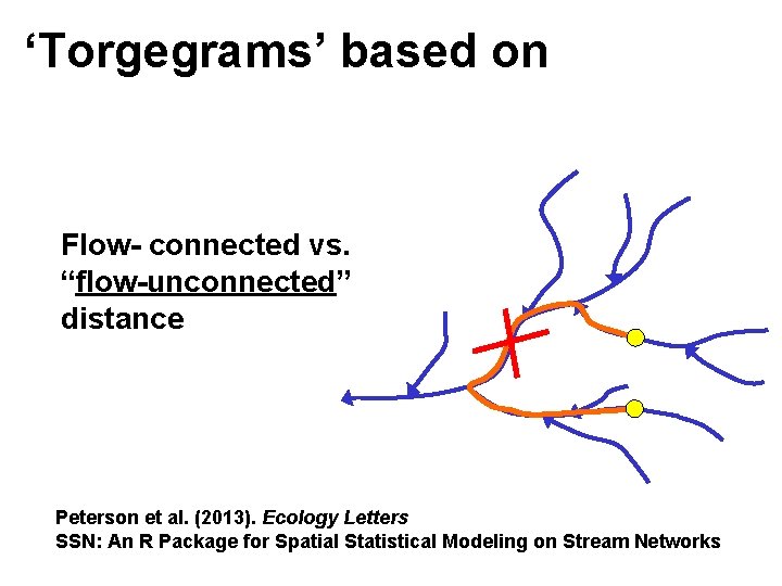
‘Torgegrams’ based on Flow- connected vs. “flow-unconnected” distance ? Peterson et al. (2013). Ecology Letters SSN: An R Package for Spatial Statistical Modeling on Stream Networks

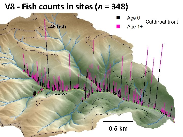
V 8 - Fish counts in sites (n = 348) Cutthroat trout 45 fish 0. 5 km

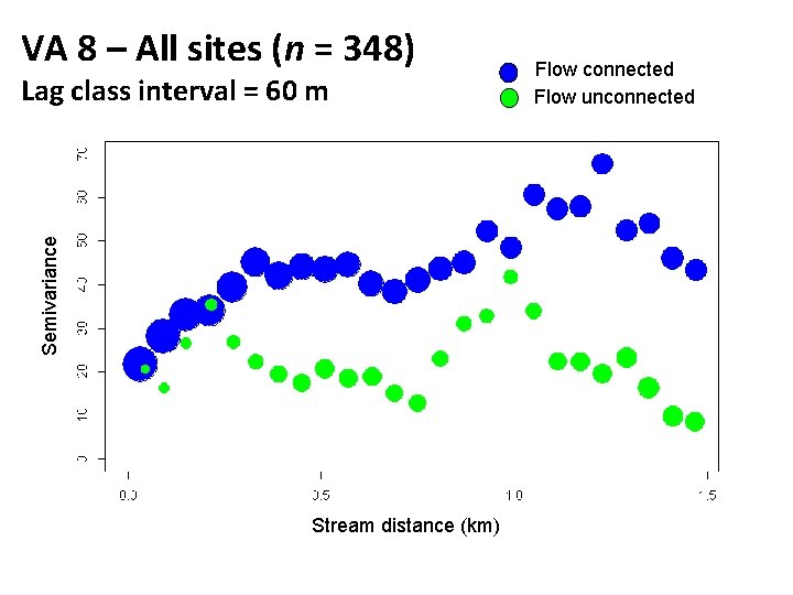
VA 8 – All sites (n = 348) Semivariance Lag class interval = 60 m Stream distance (km) Flow connected Flow unconnected

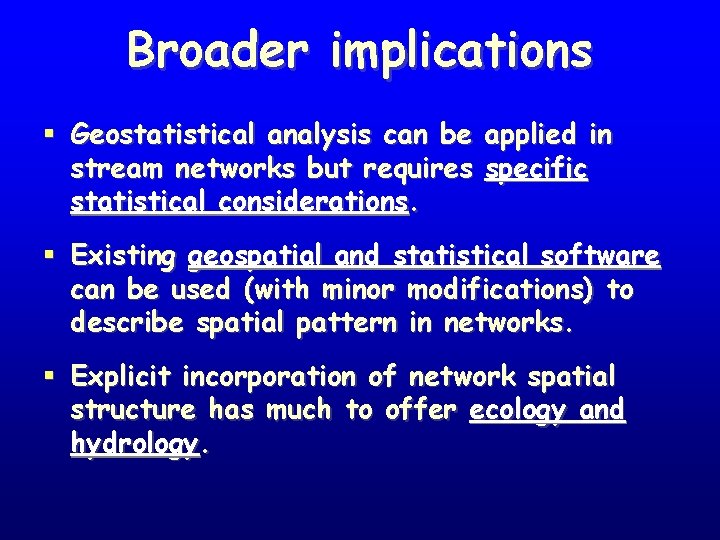
Broader implications § Geostatistical analysis can be applied in stream networks but requires specific statistical considerations. § Existing geospatial and statistical software can be used (with minor modifications) to describe spatial pattern in networks. § Explicit incorporation of network spatial structure has much to offer ecology and hydrology.

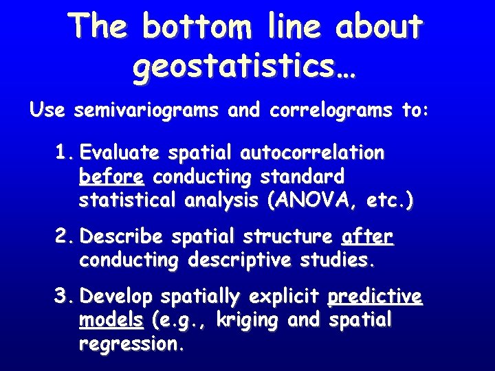
The bottom line about geostatistics… Use semivariograms and correlograms to: 1. Evaluate spatial autocorrelation before conducting standard statistical analysis (ANOVA, etc. ) 2. Describe spatial structure after conducting descriptive studies. 3. Develop spatially explicit predictive models (e. g. , kriging and spatial regression.

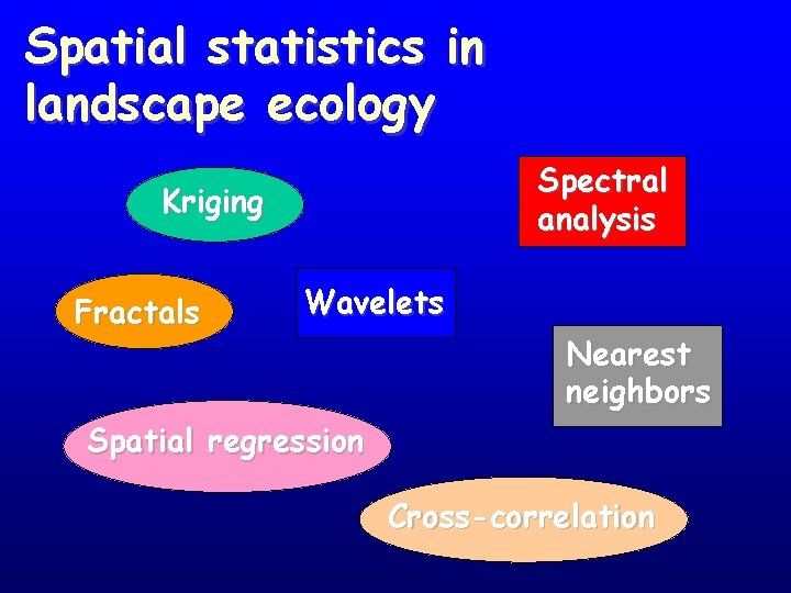
Spatial statistics in landscape ecology Spectral analysis Kriging Fractals Wavelets Nearest neighbors Spatial regression Cross-correlation

More information… Landscape Ecology Lab (Marie-Josee Fortin) http: //www. zoo. utoronto. ca/fortin Pattern Analysis, Spatial Statistics, and Geographic Exegesis (Michael Rosenberg) http: //lsweb. la. asu. edu/rosenberg/Passage GS+ (Gamma Design Software) http: //www. geostatistics. com/index. htm National Center for Ecological Analysis and Synthesis (NCEAS) http: //www. nceas. ucsb. edu/statmod Landscape Ecology Laboratory (Dean Urban and Pat Halpin) http: //www. env. duke. edu/landscape USGS Forest and Rangeland Ecosystem Science Center http: //oregonstate. edu/~torgersc

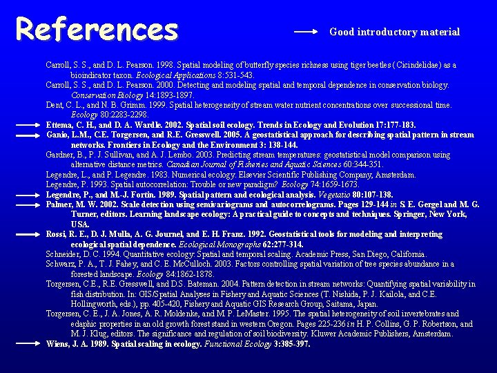
References Good introductory material Carroll, S. S. , and D. L. Pearson. 1998. Spatial modeling of butterfly species richness using tiger beetles ( Cicindelidae) as a bioindicator taxon. Ecological Applications 8: 531 -543. Carroll, S. S. , and D. L. Pearson. 2000. Detecting and modeling spatial and temporal dependence in conservation biology. Conservation Biology 14: 1893 -1897. Dent, C. L. , and N. B. Grimm. 1999. Spatial heterogeneity of stream water nutrient concentrations over successional time. Ecology 80: 2283 -2298. Ettema, C. H. , and D. A. Wardle. 2002. Spatial soil ecology. Trends in Ecology and Evolution 17: 177 -183. Ganio, L. M. , C. E. Torgersen, and R. E. Gresswell. 2005. A geostatistical approach for describing spatial pattern in stream networks. Frontiers in Ecology and the Environment 3: 138 -144. Gardner, B. , P. J. Sullivan, and A. J. Lembo. 2003. Predicting stream temperatures: geostatistical model comparison using alternative distance metrics. Canadian Journal of Fisheries and Aquatic Sciences 60: 344 -351. Legendre, L. , and P. Legendre. 1983. Numerical ecology. Elsevier Scientific Publishing Company, Amsterdam. Legendre, P. 1993. Spatial autocorrelation: Trouble or new paradigm? Ecology 74: 1659 -1673. Legendre, P. , and M. -J. Fortin. 1989. Spatial pattern and ecological analysis. Vegetatio 80: 107 -138. Palmer, M. W. 2002. Scale detection using semivariograms and autocorrelograms. Pages 129 -144 in S. E. Gergel and M. G. Turner, editors. Learning landscape ecology: A practical guide to concepts and techniques. Springer, New York, USA. Rossi, R. E. , D. J. Mulla, A. G. Journel, and E. H. Franz. 1992. Geostatistical tools for modeling and interpreting ecological spatial dependence. Ecological Monographs 62: 277 -314. Schneider, D. C. 1994. Quantitative ecology: Spatial and temporal scaling. Academic Press, San Diego, California. Schwarz, P. A. , T. J. Fahey, and C. E. Mc. Culloch. 2003. Factors controlling spatial variation of tree species abundance in a forested landscape. Ecology 84: 1862 -1878. Torgersen, C. E. , R. E. Gresswell, and D. S. Bateman. 2004. Pattern detection in stream networks: Quantifying spatial variability in fish distribution. In: GIS/Spatial Analyses in Fishery and Aquatic Sciences (T. Nishida, P. J. Kailola, and C. E. Hollingworth, eds. ), pp. 405 -420, Fishery and Aquatic GIS Research Group, Saitama, Japan. Torgersen, C. E. , J. A. Jones, A. R. Moldenke, and M. P. Le. Master. 1995. The spatial heterogeneity of soil invertebrates and edaphic properties in an old growth forest stand in western Oregon. Pages 225 -236 in H. P. Collins, G. P. Robertson, and M. J. Klug, editors. The significance and regulation of soil biodiversity. Kluwer Academic Publishers, Amsterdam. Wiens, J. A. 1989. Spatial scaling in ecology. Functional Ecology 3: 385 -397.

Acknowledgements SSN & STARS: Tools for Spatial Statistical Modeling on Stream Networks http: //www. fs. fed. us/rm/boise/AWAE/projects/Spatial. Stream. Networks. shtml