What is the WHT anyway and why are

What is the WHT anyway, and why are there so many ways to compute it? Jeremy Johnson 1, 2, 6, 24, 112, 568, 3032, 16768, …

Walsh-Hadamard Transform • y = WHTN x, N = 2 n

WHT Algorithms • Factor WHTN into a product of sparse structured matrices • Compute: y = (M 1 M 2 … Mt)x yt = Mtx … y 2 = M 2 y 3 y = M 1 y 2

Factoring the WHT Matrix • • AC BD = (A B)(C D) A B = (A I)(I B) A (B C) = (A B) C Im In = Imn WHT 2 = (WHT 2 I 2)(I 2 WHT 2)

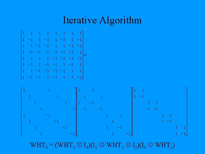
Recursive and Iterative Factorization WHT 8 = (WHT 2 I 4)(I 2 WHT 4) = (WHT 2 I 4)(I 2 ((WHT 2 I 2) (I 2 WHT 2))) = (WHT 2 I 4)(I 2 (WHT 2 I 2)) (I 2 WHT 2)) = (WHT 2 I 4)(I 2 (WHT 2 I 2)) ((I 2 I 2) WHT 2) = (WHT 2 I 4)(I 2 WHT 2 I 2) (I 4 WHT 2)

Recursive Algorithm WHT 8 = (WHT 2 I 4)(I 2 (WHT 2 I 2)(I 2 WHT 2))

WHT Algorithms • Recursive • Iterative • General

WHT Implementation • Definition/formula – N=N 1* N 2 Nt Ni=2 ni M – x=WHTN*x xb, s=(x(b), x(b+s), …x(b+(M-1)s)) • Implementation(nested loop) R=N; S=1; for i=t, …, 1 R=R/Ni WHT 2 n = for j=0, …, R-1 for k=0, …, S-1 S=S* Ni; t Õ (I i= 1 WHT 2 n i I 2 ni+1+ ··· +nt) 2 n 1+ ··· +ni-1

Partition Trees 9 Left Recursive 3 4 3 1 1 1 2 4 2 1 1 Right Recursive 2 4 1 1 Balanced 1 1 1 2 1 4 Iterative 4 1 3 1 1

Ordered Partitions • There is a 1 -1 mapping from ordered partitions of n onto (n-1)-bit binary numbers. ÞThere are 2 n-1 ordered partitions of n. 162 = 1 0 0 0 1|1 1 1 1|1 1 1+2+4+2 = 9

Enumerating Partition Trees 00 01 01 3 3 3 2 1 1 10 10 11 3 3 3 2 1 1 1

Search Space • Optimization of the WHT becomes a search, over the space of partition trees, for the fastest algorithm. • The number of trees:

Size of Search Space • Let T(z) be the generating function for Tn Tn = ( n/n 3/2), where =4+ 8 6. 8284 • Restricting to binary trees Tn = (5 n/n 3/2)

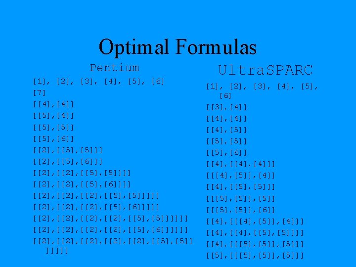
WHT Package Püschel & Johnson (ICASSP ’ 00) • Allows easy implementation of any of the possible WHT algorithms • Partition tree representation W(n)=small[n] | split[W(n 1), …W(nt)] • Tools – Measure runtime of any algorithm – Measure hardware events – Search for good implementation • Dynamic programming • Evolutionary algorithm

Histogram (n = 16, 10, 000 samples) • Wide range in performance despite equal number of arithmetic operations (n 2 n flops) • Pentium III consumes more run time (more pipeline stages) • Ultra SPARC II spans a larger range

Operation Count Theorem. Let WN be a WHT algorithm of size N. Then the number of floating point operations (flops) used by WN is Nlg(N). Proof. By induction.

Instruction Count Model A(n) = number of calls to WHT procedure = number of instructions outside loops Al(n) = Number of calls to base case of size l l = number of instructions in base case of size l Li = number of iterations of outer (i=1), middle (i=2), and outer (i=3) loop i = number of instructions in outer (i=1), middle (i=2), and outer (i=3) loop body

Small[1]. file "s_1. c" . version "01. 01" gcc 2_compiled. : . text. align 4. globl apply_small 1. type apply_small 1, @function apply_small 1: movl 8(%esp), %edx //load stride S to EDX movl 12(%esp), %eax //load x array's base address to EAX fldl (%eax) // st(0)=R 7=x[0] fldl (%eax, %edx, 8) //st(0)=R 6=x[S] fld %st(1) //st(0)=R 5=x[0] fadd %st(1), %st // R 5=x[0]+x[S] fxch %st(2) //st(0)=R 5=x[0], s(2)=R 7=x[0]+x[S] fsubp %st, %st(1) //st(0)=R 6=x[S]-x[0] ? ? ? fxch %st(1) //st(0)=R 6=x[0]+x[S], st(1)=R 7=x[S]-x[0] fstpl (%eax) //store x[0]=x[0]+x[S] fstpl (%eax, %edx, 8) //store x[0]=x[0]-x[S] ret

Recurrences

Recurrences

Histogram using Instruction Model (P 3) l = 12, l = 34, and l = 106 = 27 1 = 18, 2 = 18, and 1 = 20

Algorithm Comparison

Dynamic Programming min n 1+… + nt= n n Cost( Tn … 1 ), Tnt where Tn is the optimial tree of size n. This depends on the assumption that Cost only depends on the size of a tree and not where it is located. (true for IC, but false for runtime). For IC, the optimal tree is iterative with appropriate leaves. For runtime, DP is a good heuristic (used with binary trees).

Different Strides • Dynamic programming assumption is not true. Execution time depends on stride.