What is the correct number of break points

What is the correct number of break points hidden in a climate record? Dip. Doc. Sem – 12. December 2011

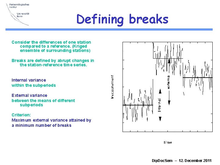
Defining breaks Consider the differences of one station compared to a reference. (Kriged ensemble of surrounding stations) Breaks are defined by abrupt changes in the station-reference time series. Internal variance within the subperiods External variance between the means of different subperiods Criterion: Maximum external variance attained by a minimum number of breaks Dip. Doc. Sem – 12. December 2011

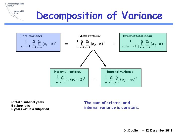
Decomposition of Variance n total number of years N subperiods ni years within a subperiod The sum of external and internal variance is constant. Dip. Doc. Sem – 12. December 2011

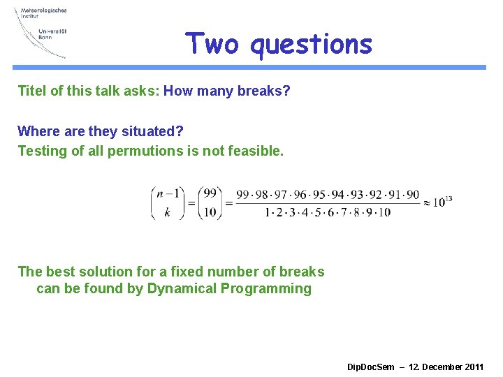
Two questions Titel of this talk asks: How many breaks? Where are they situated? Testing of all permutions is not feasible. The best solution for a fixed number of breaks can be found by Dynamical Programming Dip. Doc. Sem – 12. December 2011

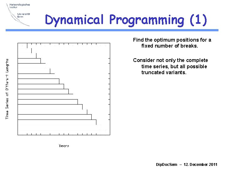
Dynamical Programming (1) Find the optimum positions for a fixed number of breaks. Consider not only the complete time series, but all possible truncated variants. Dip. Doc. Sem – 12. December 2011

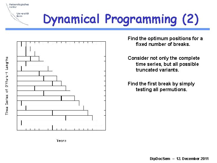
Dynamical Programming (2) Find the optimum positions for a fixed number of breaks. Consider not only the complete time series, but all possible truncated variants. Find the first break by simply testing all permutions. Dip. Doc. Sem – 12. December 2011

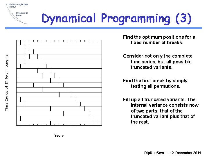
Dynamical Programming (3) Find the optimum positions for a fixed number of breaks. Consider not only the complete time series, but all possible truncated variants. Find the first break by simply testing all permutions. Fill up all truncated variants. The internal variance consists now of two parts: that of the truncated variant plus that of the rest. Dip. Doc. Sem – 12. December 2011

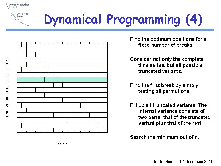
Dynamical Programming (4) Find the optimum positions for a fixed number of breaks. Consider not only the complete time series, but all possible truncated variants. Find the first break by simply testing all permutions. Fill up all truncated variants. The internal variance consists of two parts: that of the truncated variant plus that of the rest. Search the minimum out of n. Dip. Doc. Sem – 12. December 2011

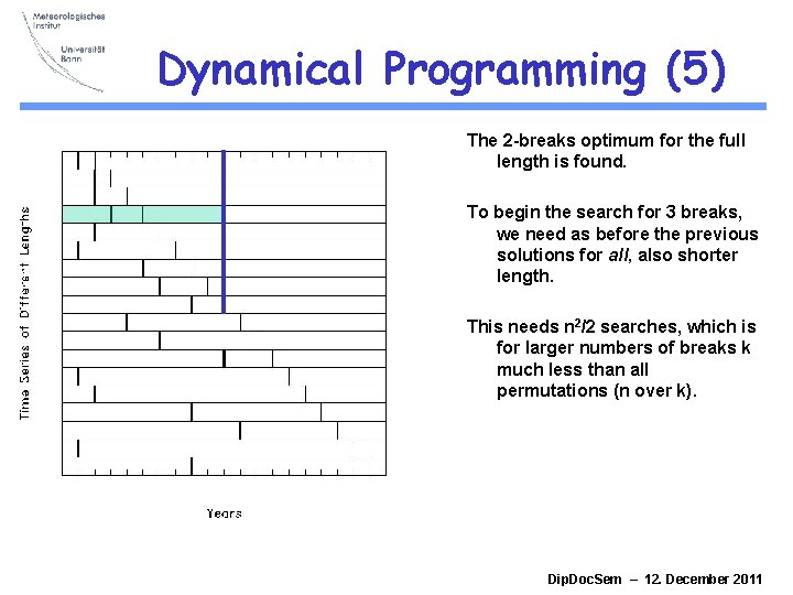
Dynamical Programming (5) The 2 -breaks optimum for the full length is found. To begin the search for 3 breaks, we need as before the previous solutions for all, also shorter length. This needs n 2/2 searches, which is for larger numbers of breaks k much less than all permutations (n over k). Dip. Doc. Sem – 12. December 2011

Position & Number Solved: The optimum positions for a fixed number of breaks are known by Dynamical Programming. Left: Find the optimum number of breaks. The external variance increase in any case with increasing number of breaks. Use as benchmark the behaviour of a random time series. Dip. Doc. Sem – 12. December 2011

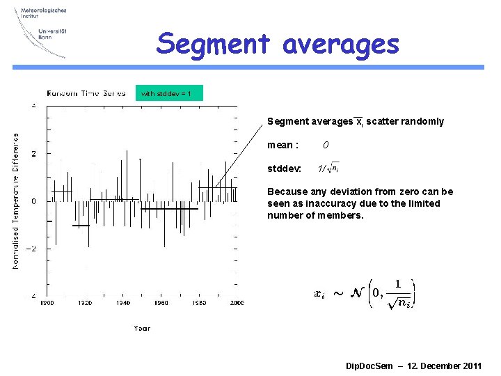
Segment averages with stddev = 1 Segment averages xi scatter randomly mean : stddev: 0 1/ Because any deviation from zero can be seen as inaccuracy due to the limited number of members. Dip. Doc. Sem – 12. December 2011

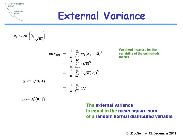
External Variance Weighted measure for the variability of the subperiods‘ means The external variance is equal to the mean square sum of a random normal distributed variable. Dip. Doc. Sem – 12. December 2011

c 2 -distribution n: k: N = k+1: [ ]: Length of time series (Number of years) Number of breaks Number of subsegments Mean of several break position permutations [varext] = (N-1)/n = k/n In average, the external variance increases linearly with k. However, we consider the best member as found by DP. varext ~ c. N 2 The external variance is chi 2 -distributed. Def. : Take N values out of N (0, 1), square and add them up. By repeating a c. N 2 -distribution is obtained. Dip. Doc. Sem – 12. December 2011

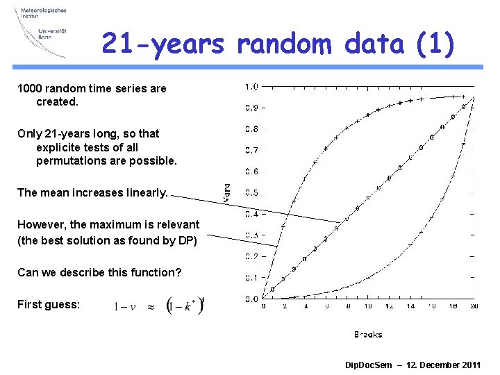
21 -years random data (1) 1000 random time series are created. Only 21 -years long, so that explicite tests of all permutations are possible. The mean increases linearly. However, the maximum is relevant (the best solution as found by DP) Can we describe this function? First guess: Dip. Doc. Sem – 12. December 2011

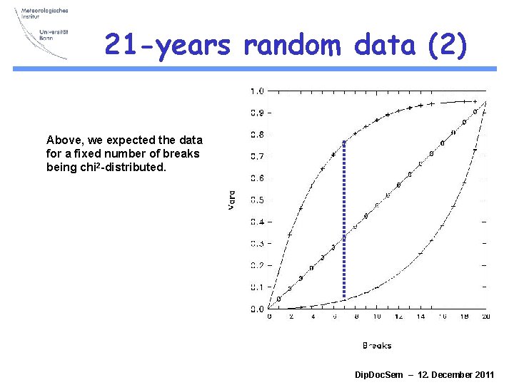
21 -years random data (2) Above, we expected the data for a fixed number of breaks being chi 2 -distributed. Dip. Doc. Sem – 12. December 2011

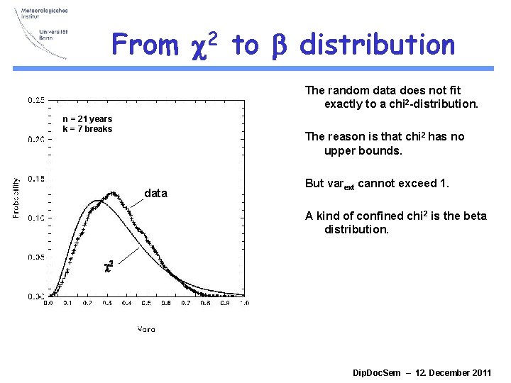
From c 2 to b distribution The random data does not fit exactly to a chi 2 -distribution. n = 21 years k = 7 breaks The reason is that chi 2 has no upper bounds. data But varext cannot exceed 1. A kind of confined chi 2 is the beta distribution. c 2 Dip. Doc. Sem – 12. December 2011

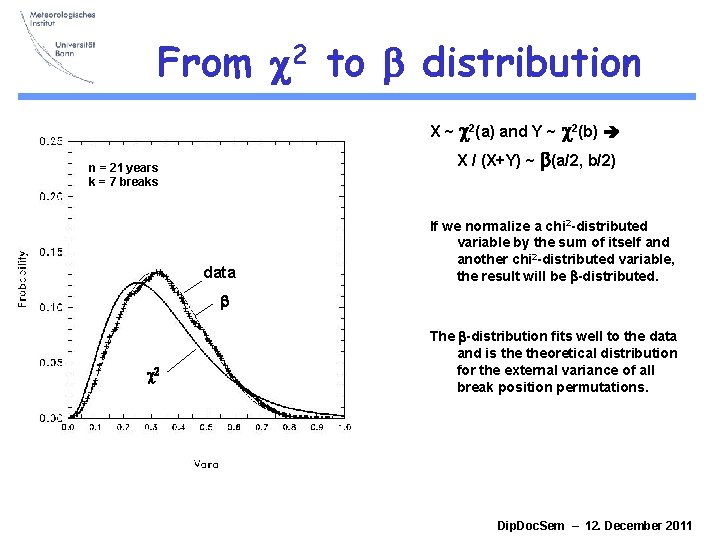
From c 2 to b distribution X ~ c 2(a) and Y ~ c 2(b) X / (X+Y) ~ b(a/2, b/2) n = 21 years k = 7 breaks data If we normalize a chi 2 -distributed variable by the sum of itself and another chi 2 -distributed variable, the result will be b-distributed. b c 2 The b-distribution fits well to the data and is theoretical distribution for the external variance of all break position permutations. Dip. Doc. Sem – 12. December 2011

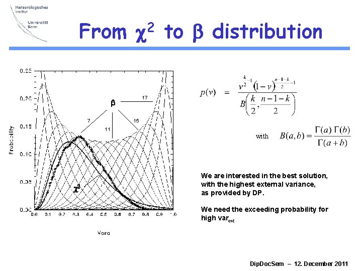
From c 2 to b distribution 17 b 7 15 11 with c 2 We are interested in the best solution, with the highest external variance, as provided by DP. We need the exceeding probability for high varext Dip. Doc. Sem – 12. December 2011

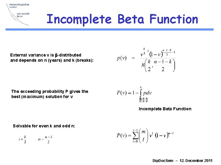
Incomplete Beta Function External variance v is b-distributed and depends on n (years) and k (breaks): The exceeding probability P gives the best (maximum) solution for v Incomplete Beta Function Solvable for even k and odd n: Dip. Doc. Sem – 12. December 2011

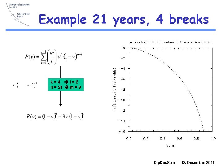
Example 21 years, 4 breaks k=4 i=2 n = 21 m = 9 Dip. Doc. Sem – 12. December 2011

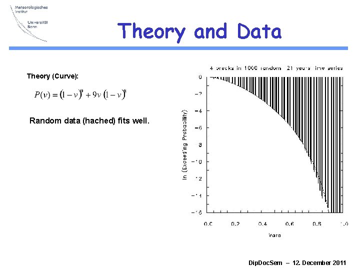
Theory and Data Theory (Curve): Random data (hached) fits well. Dip. Doc. Sem – 12. December 2011

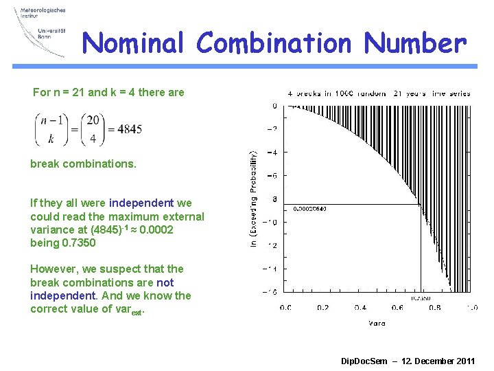
Nominal Combination Number For n = 21 and k = 4 there are break combinations. If they all were independent we could read the maximum external variance at (4845)-1 ≈ 0. 0002 being 0. 7350 However, we suspect that the break combinations are not independent. And we know the correct value of varext. Dip. Doc. Sem – 12. December 2011

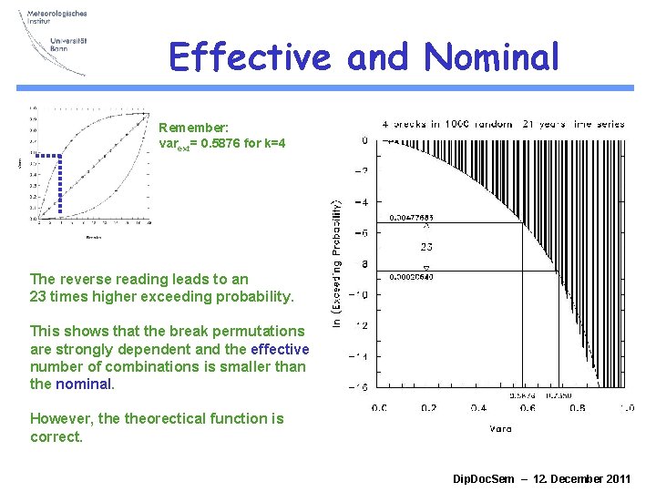
Effective and Nominal Remember: varext= 0. 5876 for k=4 The reverse reading leads to an 23 times higher exceeding probability. This shows that the break permutations are strongly dependent and the effective number of combinations is smaller than the nominal. However, theorectical function is correct. Dip. Doc. Sem – 12. December 2011

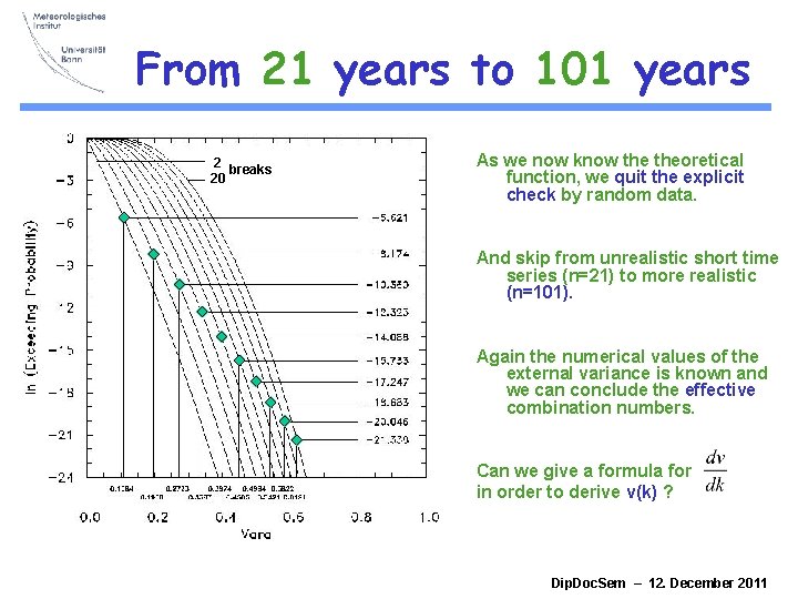
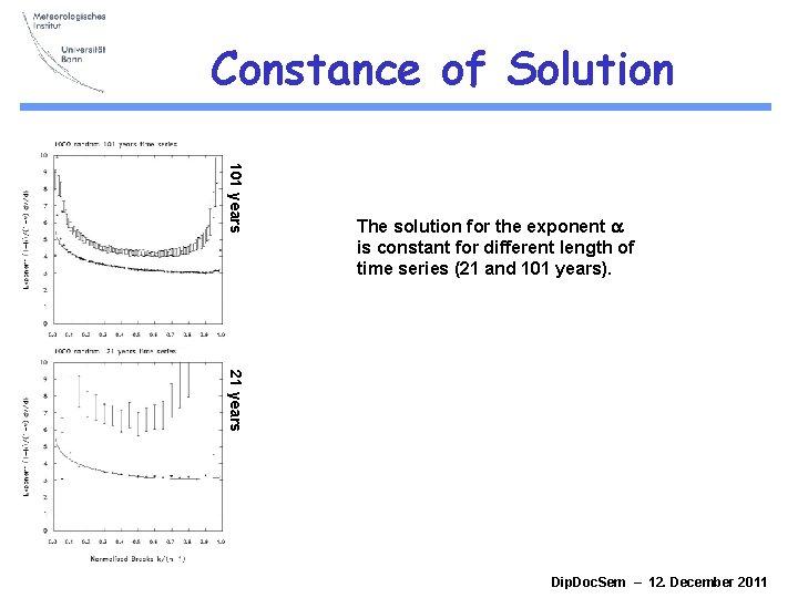
From 21 years to 101 years 2 breaks 20 As we now know theoretical function, we quit the explicit check by random data. And skip from unrealistic short time series (n=21) to more realistic (n=101). Again the numerical values of the external variance is known and we can conclude the effective combination numbers. Can we give a formula for in order to derive v(k) ? Dip. Doc. Sem – 12. December 2011

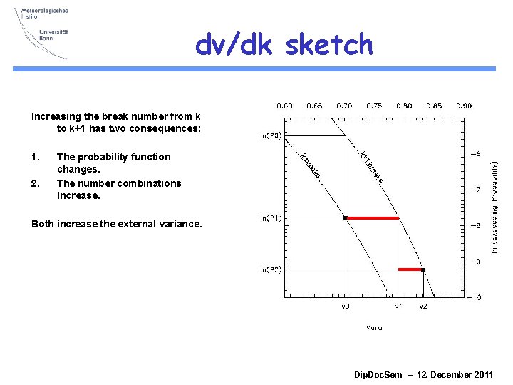
dv/dk sketch Increasing the break number from k to k+1 has two consequences: 1 b k+ s ak re 2. The probability function changes. The number combinations increase. kb 1. Both increase the external variance. Dip. Doc. Sem – 12. December 2011

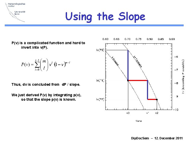
Using the Slope P(v) is a complicated function and hard to invert into v(P). 1 b k+ s ak re kb Thus, dv is concluded from d. P / slope. We just derived P(v) by integrating p(v), so that the slope p(v) is known. Dip. Doc. Sem – 12. December 2011

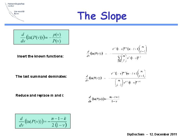
The Slope Insert the known functions: The last summand dominates: Reduce and replace m and i: Dip. Doc. Sem – 12. December 2011

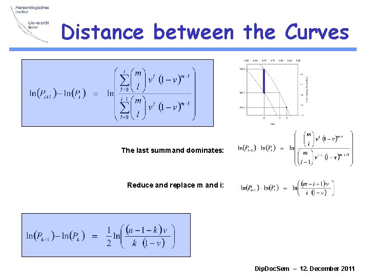
Distance between the Curves The last summand dominates: Reduce and replace m and i: Dip. Doc. Sem – 12. December 2011

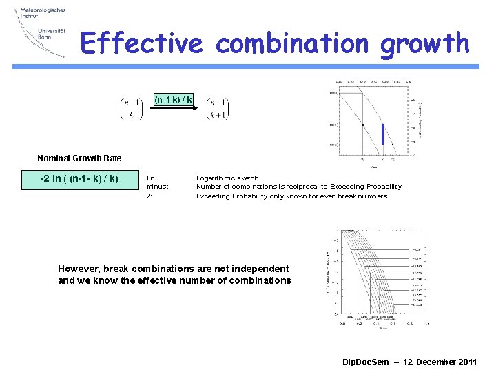
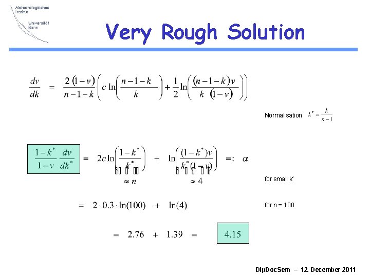
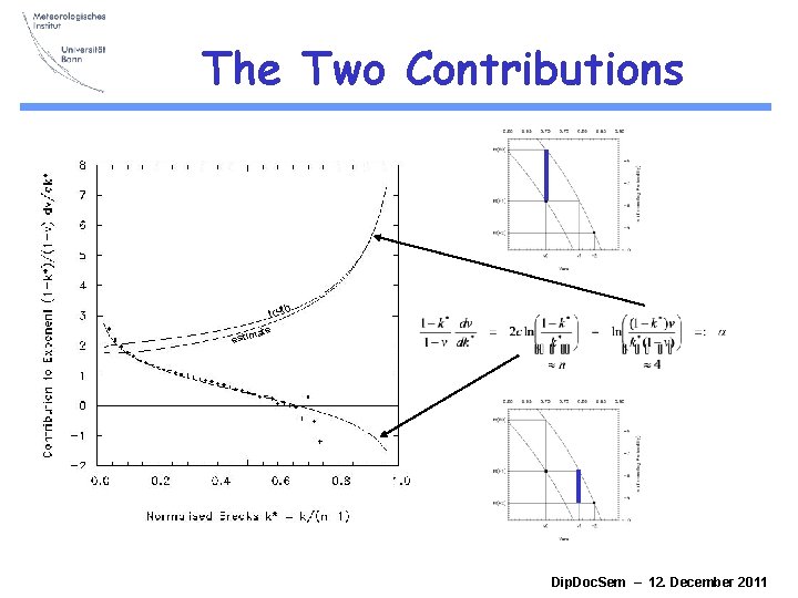
Effective combination growth (n-1 -k) / k Nominal Growth Rate -2 ln ( (n-1 - k) / k) Ln: minus: 2: Logarithmic sketch Number of combinations is reciprocal to Exceeding Probability only known for even break numbers However, break combinations are not independent and we know the effective number of combinations Dip. Doc. Sem – 12. December 2011

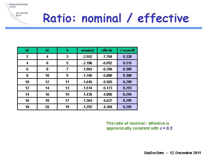
Ratio: nominal / effective k 1 k 2 k nominal effectiv c=nom/eff 2 4 3 -2. 552 -7. 784 0. 328 4 6 5 -2. 186 -6. 952 0. 315 6 8 7 -1. 963 -6. 356 0. 309 8 10 9 -1. 765 -5. 889 0. 300 10 12 11 -1. 645 -5. 503 0. 299 12 14 13 -1. 514 -5. 173 0. 293 14 16 15 -1. 435 -4. 885 0. 294 16 18 17 -1. 363 -4. 627 0. 295 18 20 19 -1. 292 -4. 394 0. 295 The ratio of nominal / effective is approximatly constant with c = 0. 3 Dip. Doc. Sem – 12. December 2011

Very Rough Solution Normalisation for small k* for n = 100 Dip. Doc. Sem – 12. December 2011

The Two Contributions h trut ate estim Dip. Doc. Sem – 12. December 2011

Exact Solution Dip. Doc. Sem – 12. December 2011

Constance of Solution 101 years The solution for the exponent a is constant for different length of time series (21 and 101 years). 21 years Dip. Doc. Sem – 12. December 2011

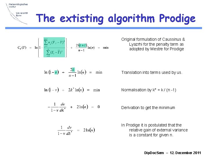
The extisting algorithm Prodige Original formulation of Caussinus & Lyazrhi for the penalty term as adopted by Mestre for Prodige Translation into terms used by us. Normalisation by k* = k / (n -1) Derivation to get the minimum In Prodige it is postulated that the relative gain of external variance is a constant for given n. Dip. Doc. Sem – 12. December 2011

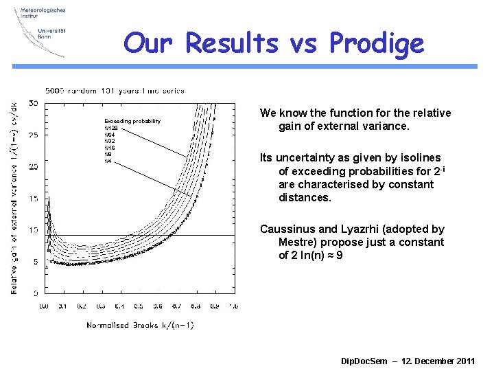
Our Results vs Prodige Exceeding probability 1/128 1/64 1/32 1/16 1/8 1/4 We know the function for the relative gain of external variance. Its uncertainty as given by isolines of exceeding probabilities for 2 -i are characterised by constant distances. Caussinus and Lyazrhi (adopted by Mestre) propose just a constant of 2 ln(n) ≈ 9 Dip. Doc. Sem – 12. December 2011

Wrong Direction n = 101 years n = 21 years Dip. Doc. Sem – 12. December 2011

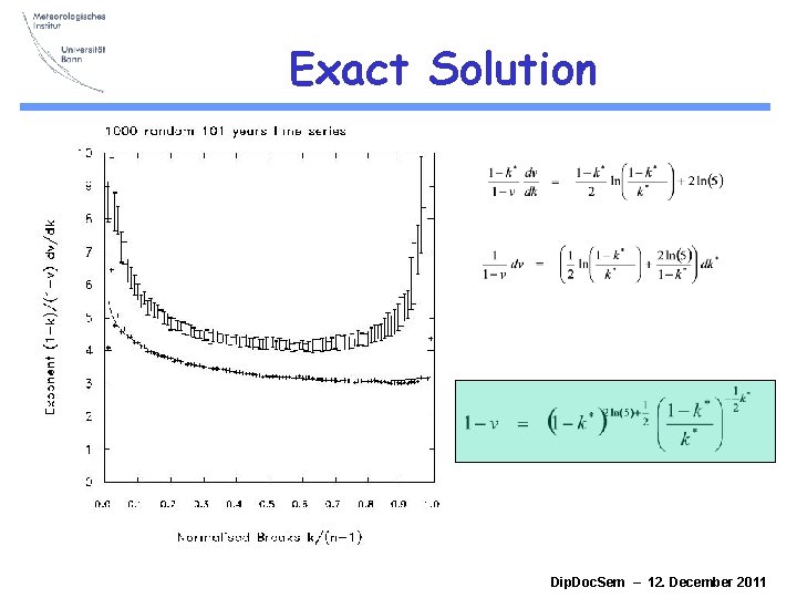
Conclusion We have found a general mathematical formulation how the external variance of a random time series is increasing when more and more breaks as given by Dynamical Programming are inserted. This is much more accurate than existing estimations and can be used in future as benchmark to define the optimum number of breaks. Dip. Doc. Sem – 12. December 2011

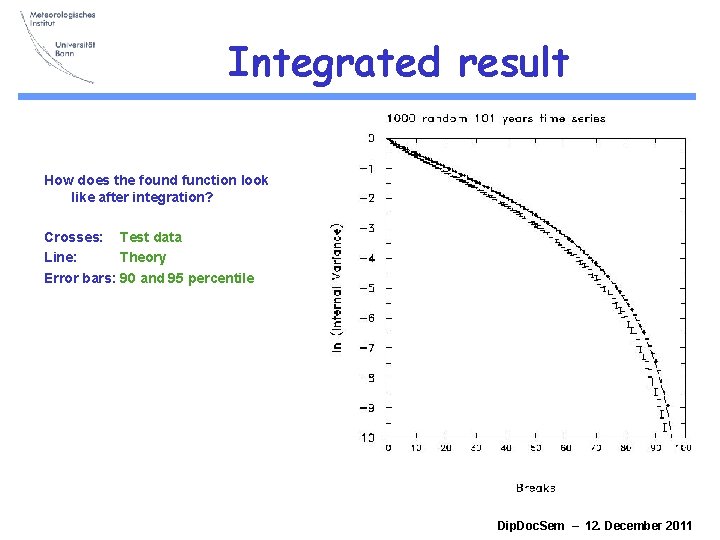
Integrated result How does the found function look like after integration? Crosses: Test data Line: Theory Error bars: 90 and 95 percentile Dip. Doc. Sem – 12. December 2011

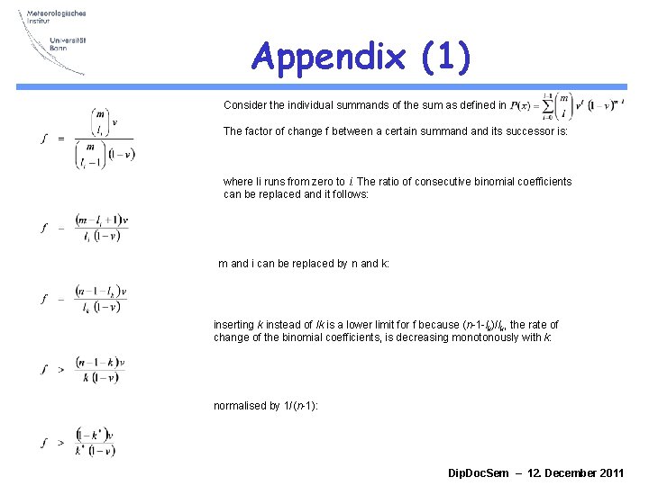
Appendix (1) Consider the individual summands of the sum as defined in The factor of change f between a certain summand its successor is: where li runs from zero to i. The ratio of consecutive binomial coefficients can be replaced and it follows: m and i can be replaced by n and k: inserting k instead of lk is a lower limit for f because (n-1 -lk)/lk, the rate of change of the binomial coefficients, is decreasing monotonously with k: normalised by 1/(n-1): Dip. Doc. Sem – 12. December 2011

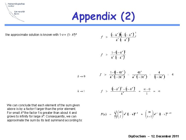
Appendix (2) the approximate solution is known with 1 -v = (1 - k*)4 We can conclude that each element of the sum given above is by a factor f larger than the prior element. For small k* the factor f is greater than about 4 and grows to infinity for large k*. Consequently, we can approximate the sum by its last summand according to: Dip. Doc. Sem – 12. December 2011

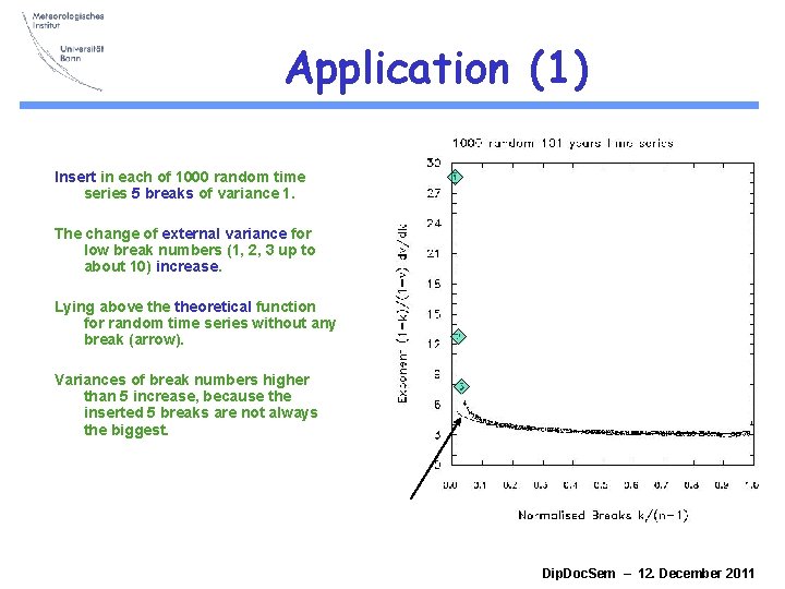
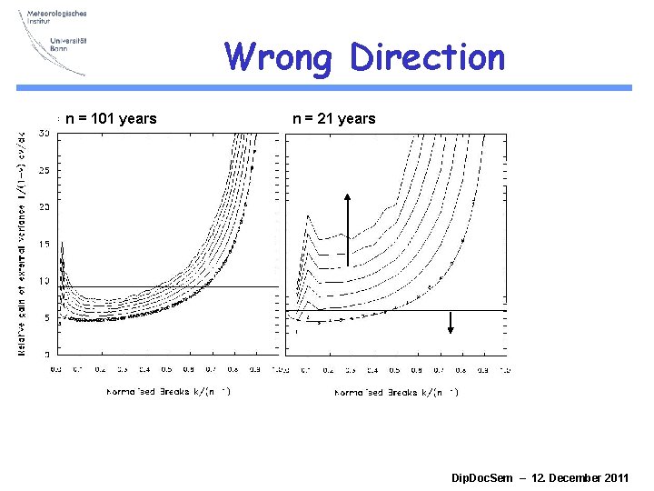
Application (1) Insert in each of 1000 random time series 5 breaks of variance 1. The change of external variance for low break numbers (1, 2, 3 up to about 10) increase. Lying above theoretical function for random time series without any break (arrow). Variances of break numbers higher than 5 increase, because the inserted 5 breaks are not always the biggest. Dip. Doc. Sem – 12. December 2011

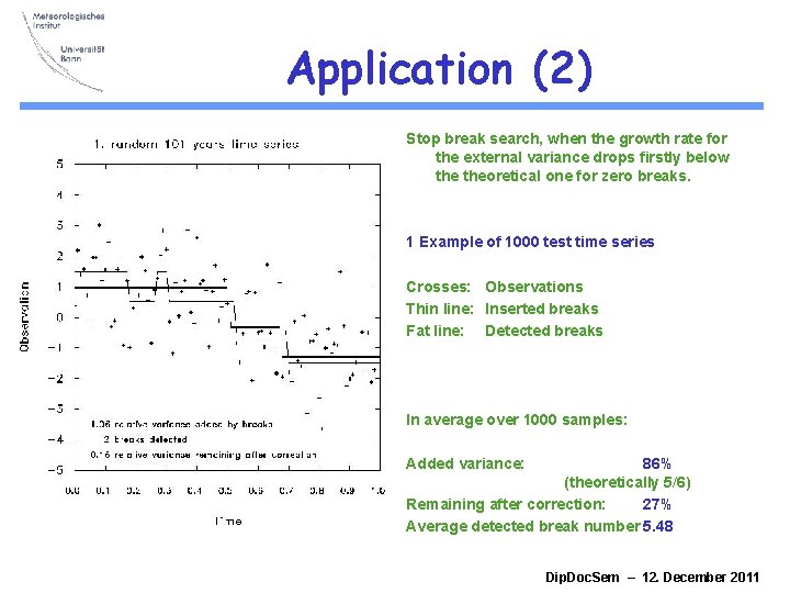
Application (2) Stop break search, when the growth rate for the external variance drops firstly below theoretical one for zero breaks. 1 Example of 1000 test time series Crosses: Observations Thin line: Inserted breaks Fat line: Detected breaks In average over 1000 samples: Added variance: 86% (theoretically 5/6) Remaining after correction: 27% Average detected break number 5. 48 Dip. Doc. Sem – 12. December 2011