What is Statistics Statistics The science of collecting

What is Statistics? Statistics The science of collecting, organizing, analyzing, and interpreting data in order to make decisions. Larson/Farber 4 th ed. 1

What is Data? Data Consist of information coming from observations, counts, measurements, or responses. Larson/Farber 4 th ed. 2

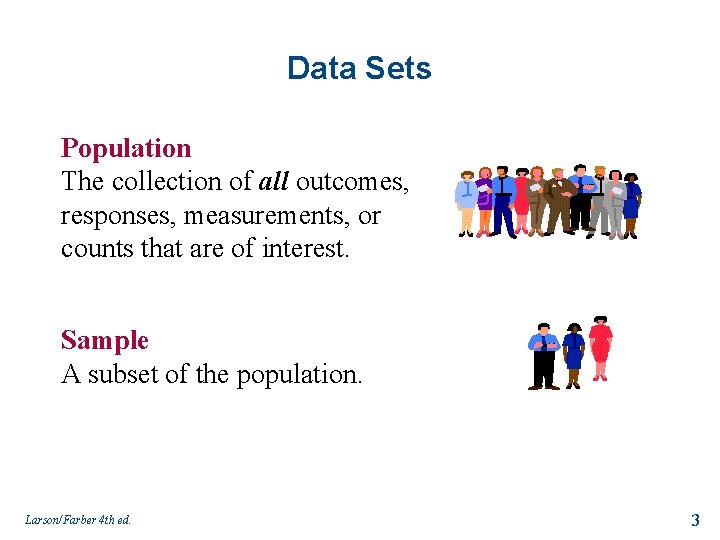
Data Sets Population The collection of all outcomes, responses, measurements, or counts that are of interest. Sample A subset of the population. Larson/Farber 4 th ed. 3

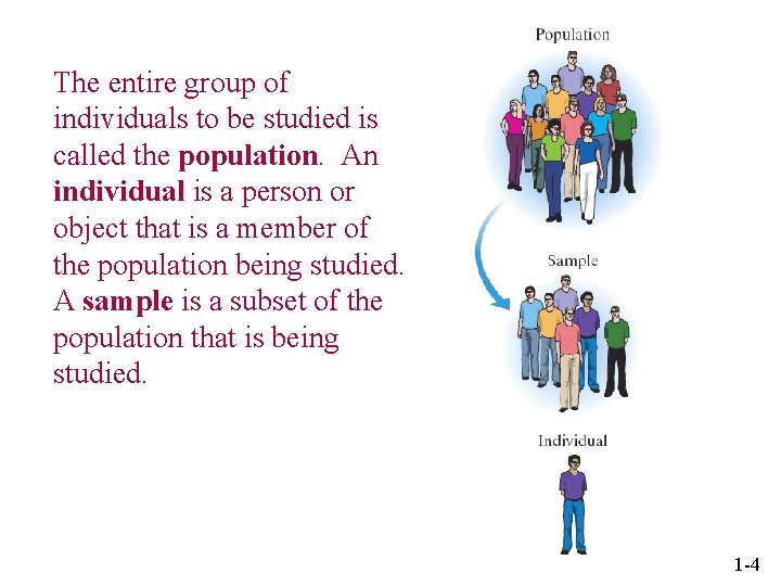
The entire group of individuals to be studied is called the population. An individual is a person or object that is a member of the population being studied. A sample is a subset of the population that is being studied. 1 -4

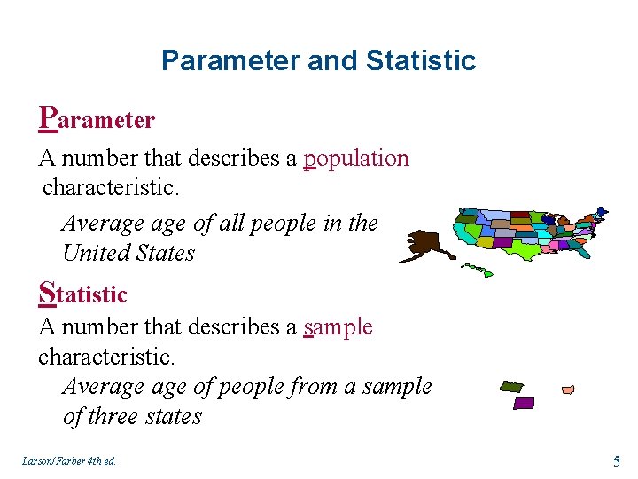
Parameter and Statistic Parameter A number that describes a population characteristic. Average of all people in the United States Statistic A number that describes a sample characteristic. Average of people from a sample of three states Larson/Farber 4 th ed. 5

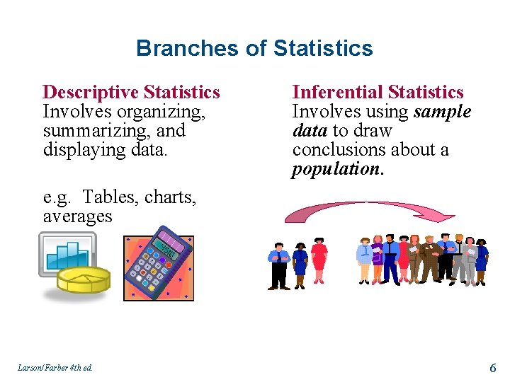
Branches of Statistics Descriptive Statistics Involves organizing, summarizing, and displaying data. Inferential Statistics Involves using sample data to draw conclusions about a population. e. g. Tables, charts, averages Larson/Farber 4 th ed. 6

Section 1. 2 Data Classification Larson/Farber 4 th ed. 7

Qualitative or Categorical variables allow for classification of individuals based on some attribute or characteristic. Quantitative variables provide numerical measures of individuals. Arithmetic operations such as addition and subtraction can be performed on the values of the quantitative variable and provide meaningful results. 1 -8

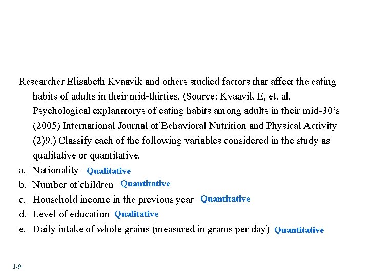
Researcher Elisabeth Kvaavik and others studied factors that affect the eating habits of adults in their mid-thirties. (Source: Kvaavik E, et. al. Psychological explanatorys of eating habits among adults in their mid-30’s (2005) International Journal of Behavioral Nutrition and Physical Activity (2)9. ) Classify each of the following variables considered in the study as qualitative or quantitative. a. Nationality Qualitative b. Number of children Quantitative c. Household income in the previous year Quantitative d. Level of education Qualitative e. Daily intake of whole grains (measured in grams per day) Quantitative 1 -9

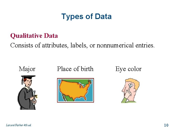
Types of Data Qualitative Data Consists of attributes, labels, or nonnumerical entries. Major Larson/Farber 4 th ed. Place of birth Eye color 10

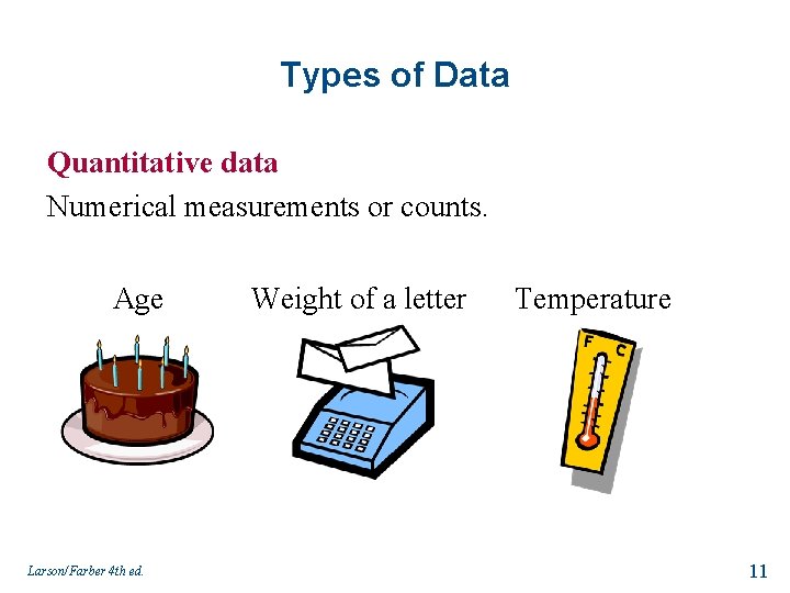
Types of Data Quantitative data Numerical measurements or counts. Age Larson/Farber 4 th ed. Weight of a letter Temperature 11

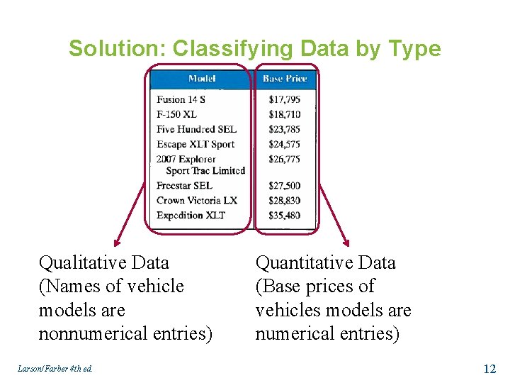
Solution: Classifying Data by Type Qualitative Data (Names of vehicle models are nonnumerical entries) Larson/Farber 4 th ed. Quantitative Data (Base prices of vehicles models are numerical entries) 12

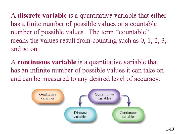
A discrete variable is a quantitative variable that either has a finite number of possible values or a countable number of possible values. The term “countable” means the values result from counting such as 0, 1, 2, 3, and so on. A continuous variable is a quantitative variable that has an infinite number of possible values it can take on and can be measured to any desired level of accuracy. 1 -13

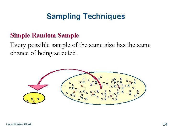
Sampling Techniques Simple Random Sample Every possible sample of the same size has the same chance of being selected. x xxxxx x x x xx xx x x x x xx x x xx x x xxxx x x x x x x xx x Larson/Farber 4 th ed. 14

Simple Random Sample • Random numbers can be generated by a random number table, a software program or a calculator. • Assign a number to each member of the population. • Members of the population that correspond to these numbers become members of the sample. Larson/Farber 4 th ed. 15

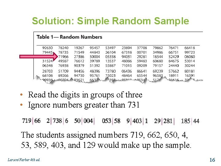
Solution: Simple Random Sample • Read the digits in groups of three • Ignore numbers greater than 731 The students assigned numbers 719, 662, 650, 4, 53, 589, 403, and 129 would make up the sample. Larson/Farber 4 th ed. 16

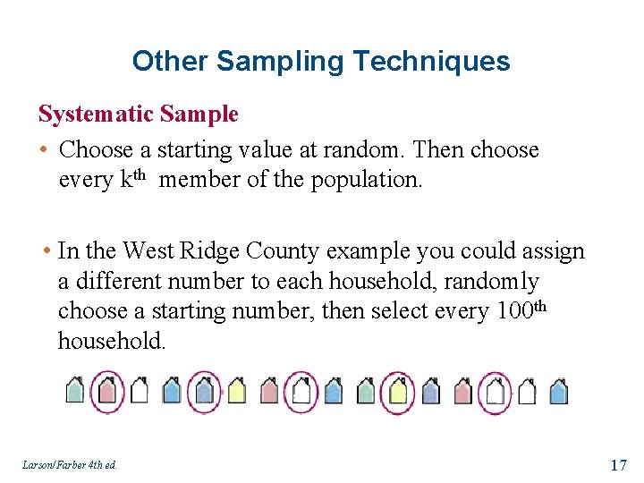
Other Sampling Techniques Systematic Sample • Choose a starting value at random. Then choose every kth member of the population. • In the West Ridge County example you could assign a different number to each household, randomly choose a starting number, then select every 100 th household. Larson/Farber 4 th ed. 17

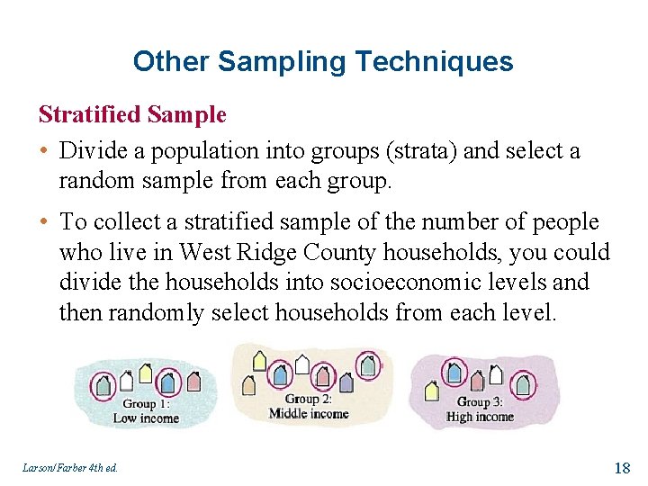
Other Sampling Techniques Stratified Sample • Divide a population into groups (strata) and select a random sample from each group. • To collect a stratified sample of the number of people who live in West Ridge County households, you could divide the households into socioeconomic levels and then randomly select households from each level. Larson/Farber 4 th ed. 18

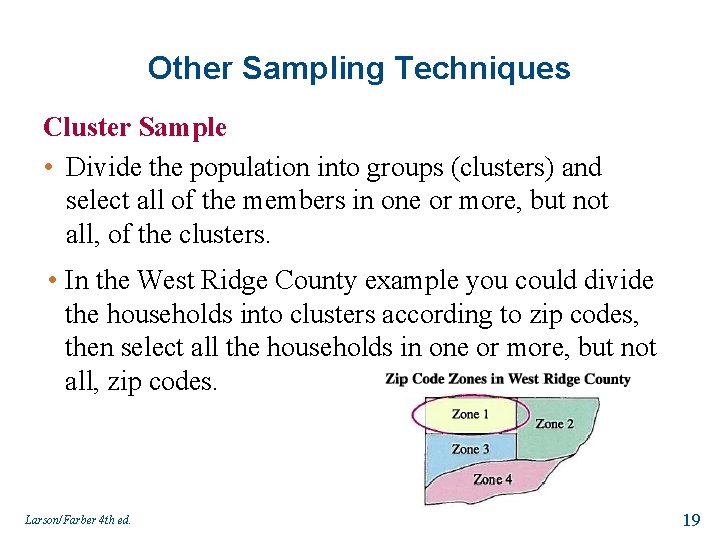
Other Sampling Techniques Cluster Sample • Divide the population into groups (clusters) and select all of the members in one or more, but not all, of the clusters. • In the West Ridge County example you could divide the households into clusters according to zip codes, then select all the households in one or more, but not all, zip codes. Larson/Farber 4 th ed. 19

A convenience sample is one in which the individuals in the sample are easily obtained. Any studies that use this type of sampling generally have results that are suspect. Results should be looked upon with extreme skepticism. 1 -20

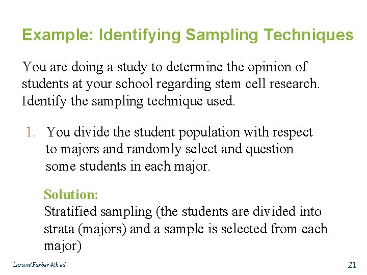
Example: Identifying Sampling Techniques You are doing a study to determine the opinion of students at your school regarding stem cell research. Identify the sampling technique used. 1. You divide the student population with respect to majors and randomly select and question some students in each major. Solution: Stratified sampling (the students are divided into strata (majors) and a sample is selected from each major) Larson/Farber 4 th ed. 21

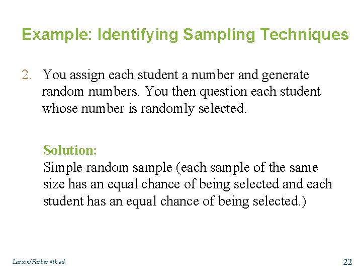
Example: Identifying Sampling Techniques 2. You assign each student a number and generate random numbers. You then question each student whose number is randomly selected. Solution: Simple random sample (each sample of the same size has an equal chance of being selected and each student has an equal chance of being selected. ) Larson/Farber 4 th ed. 22

Descriptive Statistics Measures of Central Tendency Larson/Farber 4 th ed. 23

Measures of Central Tendency Measure of central tendency • A value that represents a typical, or central, entry of a data set. • Most common measures of central tendency: § Mean § Median § Mode Larson/Farber 4 th ed. 24

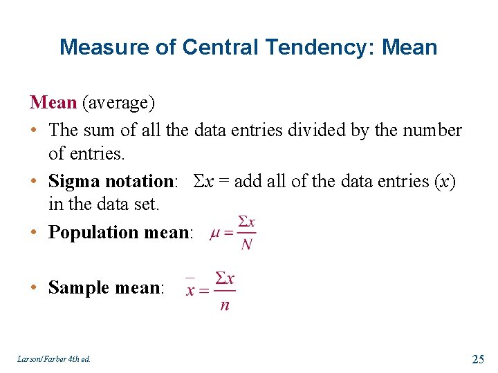
Measure of Central Tendency: Mean (average) • The sum of all the data entries divided by the number of entries. • Sigma notation: Σx = add all of the data entries (x) in the data set. • Population mean: • Sample mean: Larson/Farber 4 th ed. 25

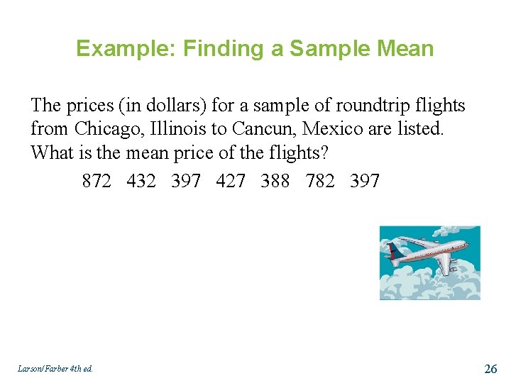
Example: Finding a Sample Mean The prices (in dollars) for a sample of roundtrip flights from Chicago, Illinois to Cancun, Mexico are listed. What is the mean price of the flights? 872 432 397 427 388 782 397 Larson/Farber 4 th ed. 26

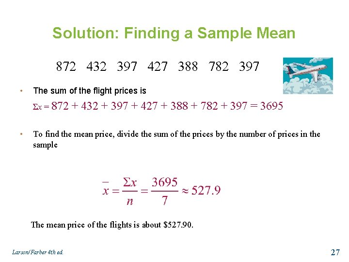
Solution: Finding a Sample Mean 872 432 397 427 388 782 397 • The sum of the flight prices is Σx = 872 • + 432 + 397 + 427 + 388 + 782 + 397 = 3695 To find the mean price, divide the sum of the prices by the number of prices in the sample The mean price of the flights is about $527. 90. Larson/Farber 4 th ed. 27

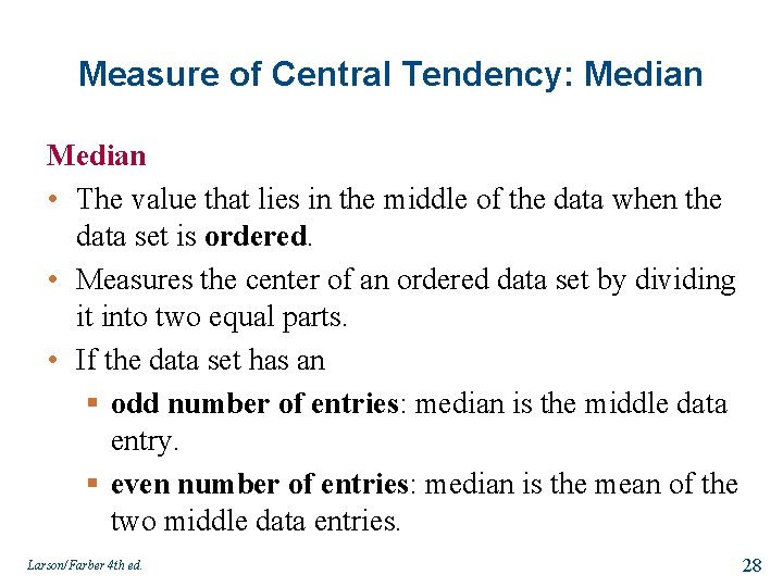
Measure of Central Tendency: Median • The value that lies in the middle of the data when the data set is ordered. • Measures the center of an ordered data set by dividing it into two equal parts. • If the data set has an § odd number of entries: median is the middle data entry. § even number of entries: median is the mean of the two middle data entries. Larson/Farber 4 th ed. 28

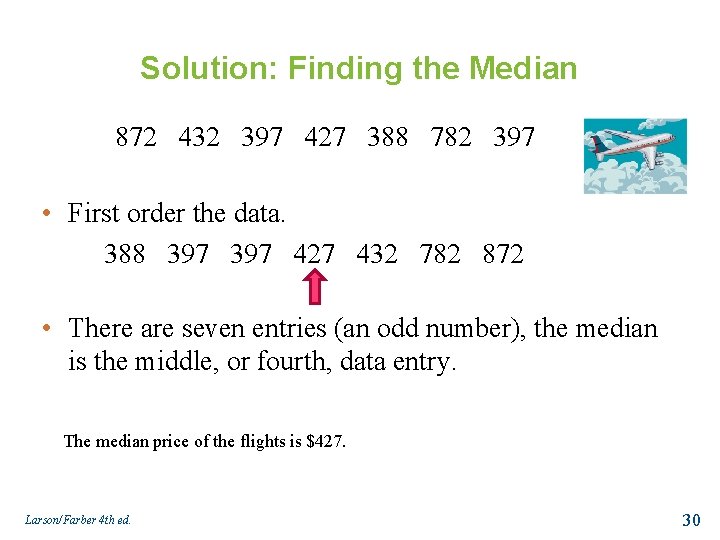
Example: Finding the Median The prices (in dollars) for a sample of roundtrip flights from Chicago, Illinois to Cancun, Mexico are listed. Find the median of the flight prices. 872 432 397 427 388 782 397 Larson/Farber 4 th ed. 29

Solution: Finding the Median 872 432 397 427 388 782 397 • First order the data. 388 397 427 432 782 872 • There are seven entries (an odd number), the median is the middle, or fourth, data entry. The median price of the flights is $427. Larson/Farber 4 th ed. 30

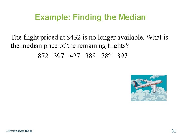
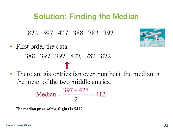
Example: Finding the Median The flight priced at $432 is no longer available. What is the median price of the remaining flights? 872 397 427 388 782 397 Larson/Farber 4 th ed. 31

Solution: Finding the Median 872 397 427 388 782 397 • First order the data. 388 397 427 782 872 • There are six entries (an even number), the median is the mean of the two middle entries. The median price of the flights is $412. Larson/Farber 4 th ed. 32

Measure of Central Tendency: Mode • The data entry that occurs with the greatest frequency. • If no entry is repeated the data set has no mode. • If two entries occur with the same greatest frequency, each entry is a mode (bimodal). Larson/Farber 4 th ed. 33

Example: Finding the Mode The prices (in dollars) for a sample of roundtrip flights from Chicago, Illinois to Cancun, Mexico are listed. Find the mode of the flight prices. 872 432 397 427 388 782 397 Larson/Farber 4 th ed. 34

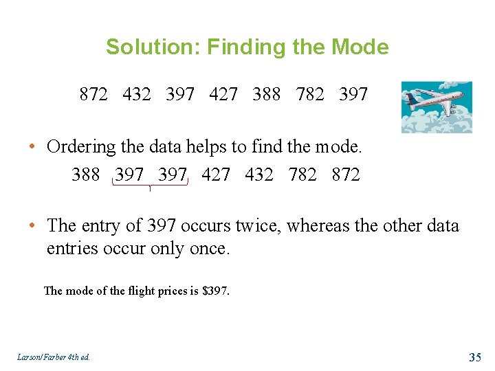
Solution: Finding the Mode 872 432 397 427 388 782 397 • Ordering the data helps to find the mode. 388 397 427 432 782 872 • The entry of 397 occurs twice, whereas the other data entries occur only once. The mode of the flight prices is $397. Larson/Farber 4 th ed. 35

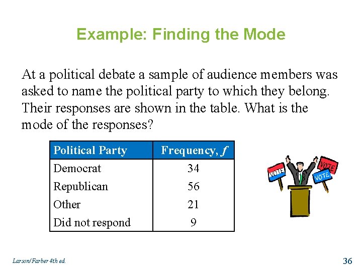
Example: Finding the Mode At a political debate a sample of audience members was asked to name the political party to which they belong. Their responses are shown in the table. What is the mode of the responses? Political Party Democrat Republican Other Frequency, f 34 56 21 Did not respond 9 Larson/Farber 4 th ed. 36

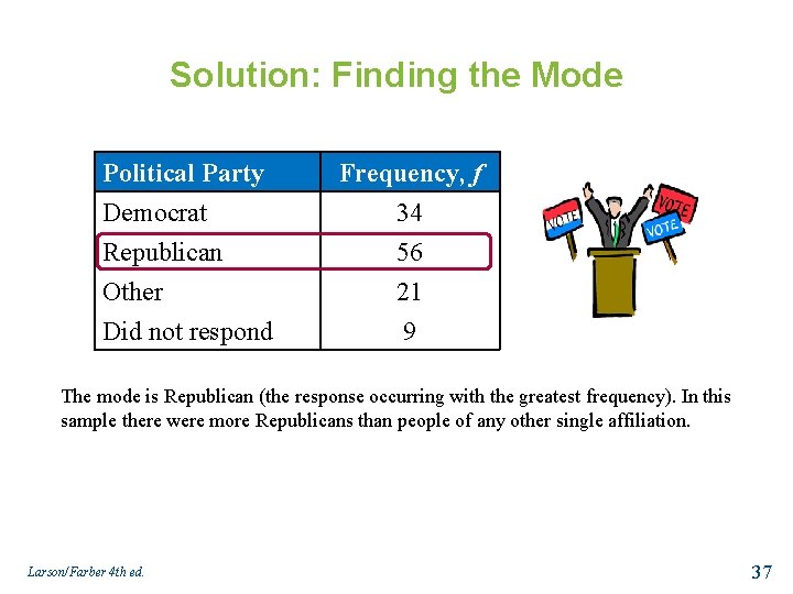
Solution: Finding the Mode Political Party Democrat Republican Other Frequency, f 34 56 21 Did not respond 9 The mode is Republican (the response occurring with the greatest frequency). In this sample there were more Republicans than people of any other single affiliation. Larson/Farber 4 th ed. 37

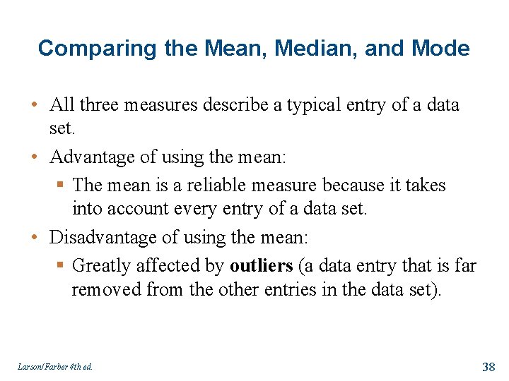
Comparing the Mean, Median, and Mode • All three measures describe a typical entry of a data set. • Advantage of using the mean: § The mean is a reliable measure because it takes into account every entry of a data set. • Disadvantage of using the mean: § Greatly affected by outliers (a data entry that is far removed from the other entries in the data set). Larson/Farber 4 th ed. 38

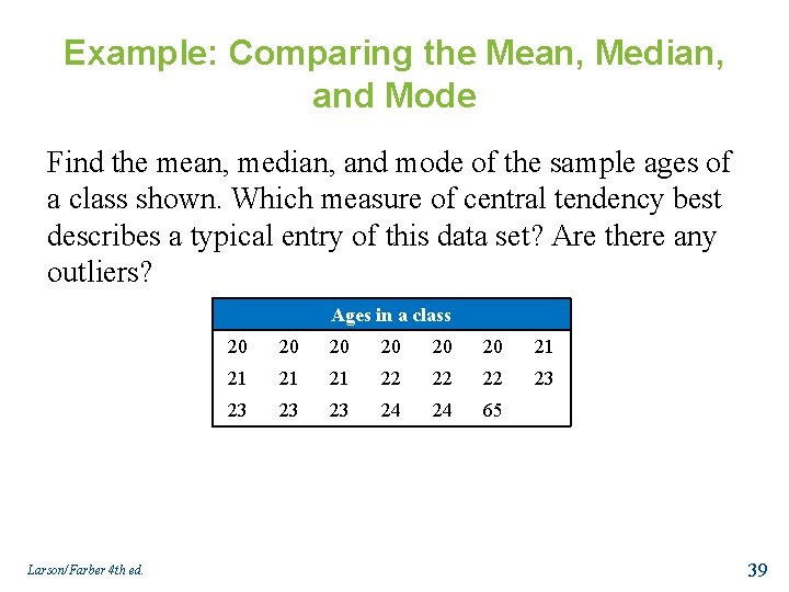
Example: Comparing the Mean, Median, and Mode Find the mean, median, and mode of the sample ages of a class shown. Which measure of central tendency best describes a typical entry of this data set? Are there any outliers? Ages in a class Larson/Farber 4 th ed. 20 20 20 21 21 22 22 22 23 23 24 24 65 39

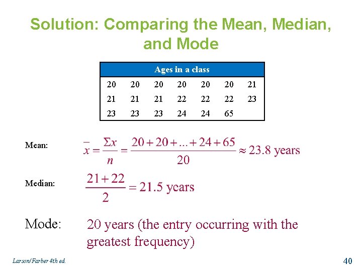
Solution: Comparing the Mean, Median, and Mode Ages in a class 20 20 20 21 21 22 22 22 23 23 24 24 65 Mean: Median: Mode: Larson/Farber 4 th ed. 20 years (the entry occurring with the greatest frequency) 40

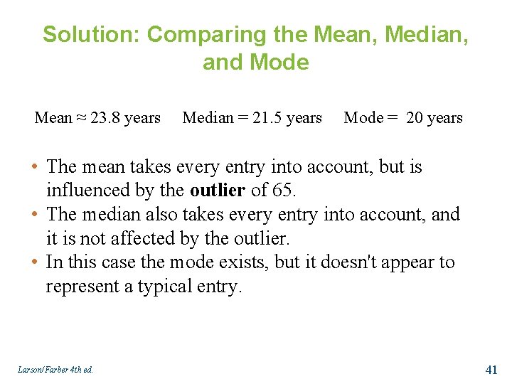
Solution: Comparing the Mean, Median, and Mode Mean ≈ 23. 8 years Median = 21. 5 years Mode = 20 years • The mean takes every entry into account, but is influenced by the outlier of 65. • The median also takes every entry into account, and it is not affected by the outlier. • In this case the mode exists, but it doesn't appear to represent a typical entry. Larson/Farber 4 th ed. 41

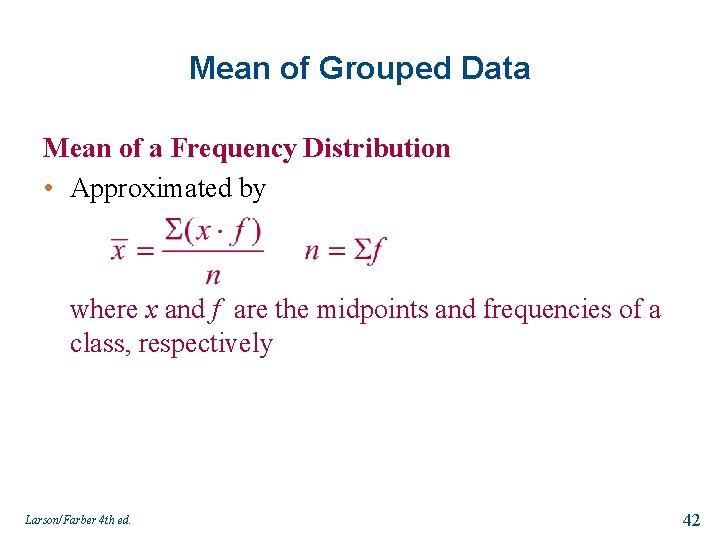
Mean of Grouped Data Mean of a Frequency Distribution • Approximated by where x and f are the midpoints and frequencies of a class, respectively Larson/Farber 4 th ed. 42

Section 2. 3 Summary • Determined the mean, median, and mode of a population and of a sample • Determined the weighted mean of a data set and the mean of a frequency distribution • Described the shape of a distribution as symmetric, uniform, or skewed and compared the mean and median for each Larson/Farber 4 th ed. 43

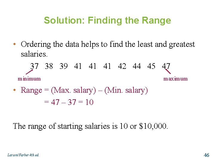
Range • The difference between the maximum and minimum data entries in the set. • The data must be quantitative. • Range = (Max. data entry) – (Min. data entry) Larson/Farber 4 th ed. 44

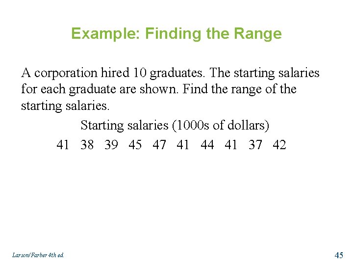
Example: Finding the Range A corporation hired 10 graduates. The starting salaries for each graduate are shown. Find the range of the starting salaries. Starting salaries (1000 s of dollars) 41 38 39 45 47 41 44 41 37 42 Larson/Farber 4 th ed. 45

Solution: Finding the Range • Ordering the data helps to find the least and greatest salaries. 37 38 39 41 41 41 42 44 45 47 minimum maximum • Range = (Max. salary) – (Min. salary) = 47 – 37 = 10 The range of starting salaries is 10 or $10, 000. Larson/Farber 4 th ed. 46

Section 2. 5 Measures of Position Larson/Farber 4 th ed. 47

Section 2. 5 Objectives • • • Determine the quartiles of a data set Determine the interquartile range of a data set Create a box-and-whisker plot Interpret other fractiles such as percentiles Determine and interpret the standard score (z-score) Larson/Farber 4 th ed. 48

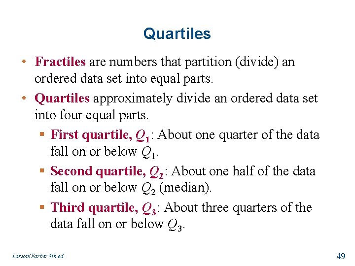
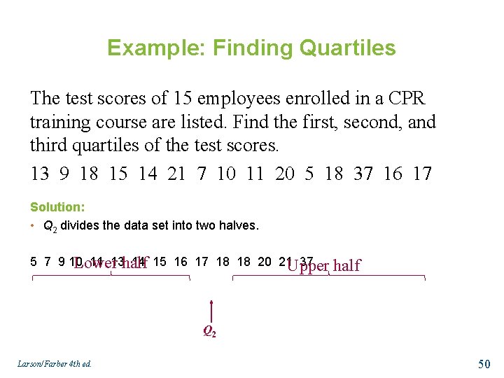
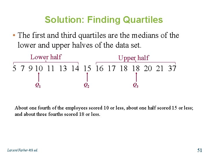
Quartiles • Fractiles are numbers that partition (divide) an ordered data set into equal parts. • Quartiles approximately divide an ordered data set into four equal parts. § First quartile, Q 1: About one quarter of the data fall on or below Q 1. § Second quartile, Q 2: About one half of the data fall on or below Q 2 (median). § Third quartile, Q 3: About three quarters of the data fall on or below Q 3. Larson/Farber 4 th ed. 49

Example: Finding Quartiles The test scores of 15 employees enrolled in a CPR training course are listed. Find the first, second, and third quartiles of the test scores. 13 9 18 15 14 21 7 10 11 20 5 18 37 16 17 Solution: • Q 2 divides the data set into two halves. 5 7 9 10 11 13 half 14 15 16 17 18 18 20 21 Upper 37 Lower half Q 2 Larson/Farber 4 th ed. 50

Solution: Finding Quartiles • The first and third quartiles are the medians of the lower and upper halves of the data set. Lower half Upper half 5 7 9 10 11 13 14 15 16 17 18 18 20 21 37 Q 1 Q 2 Q 3 About one fourth of the employees scored 10 or less, about one half scored 15 or less; and about three fourths scored 18 or less. Larson/Farber 4 th ed. 51

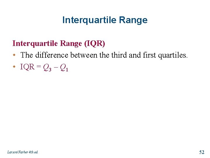
Interquartile Range (IQR) • The difference between the third and first quartiles. • IQR = Q 3 – Q 1 Larson/Farber 4 th ed. 52

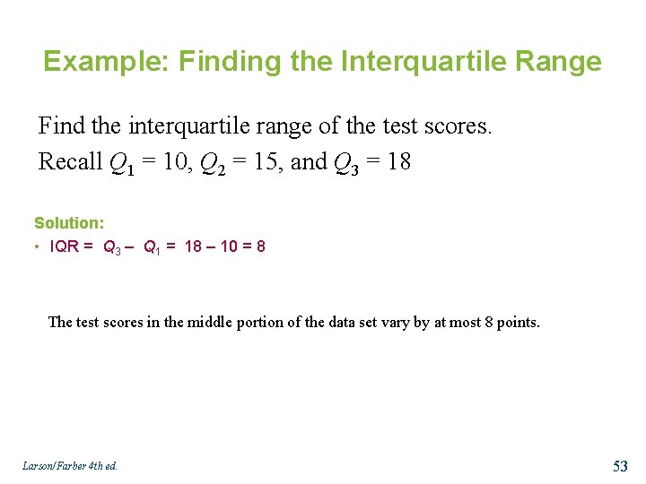
Example: Finding the Interquartile Range Find the interquartile range of the test scores. Recall Q 1 = 10, Q 2 = 15, and Q 3 = 18 Solution: • IQR = Q 3 – Q 1 = 18 – 10 = 8 The test scores in the middle portion of the data set vary by at most 8 points. Larson/Farber 4 th ed. 53

Box-and-Whisker Plot Box-and-whisker plot • Exploratory data analysis tool. • Highlights important features of a data set. • Requires (five-number summary): § Minimum entry § First quartile Q 1 § Median Q 2 § Third quartile Q 3 § Maximum entry Larson/Farber 4 th ed. 54

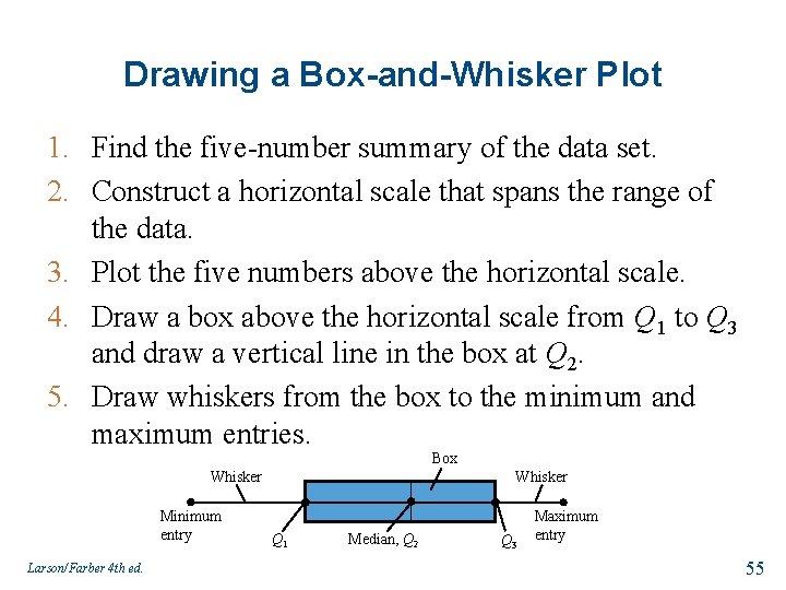
Drawing a Box-and-Whisker Plot 1. Find the five-number summary of the data set. 2. Construct a horizontal scale that spans the range of the data. 3. Plot the five numbers above the horizontal scale. 4. Draw a box above the horizontal scale from Q 1 to Q 3 and draw a vertical line in the box at Q 2. 5. Draw whiskers from the box to the minimum and maximum entries. Box Whisker Minimum entry Larson/Farber 4 th ed. Whisker Q 1 Median, Q 2 Q 3 Maximum entry 55

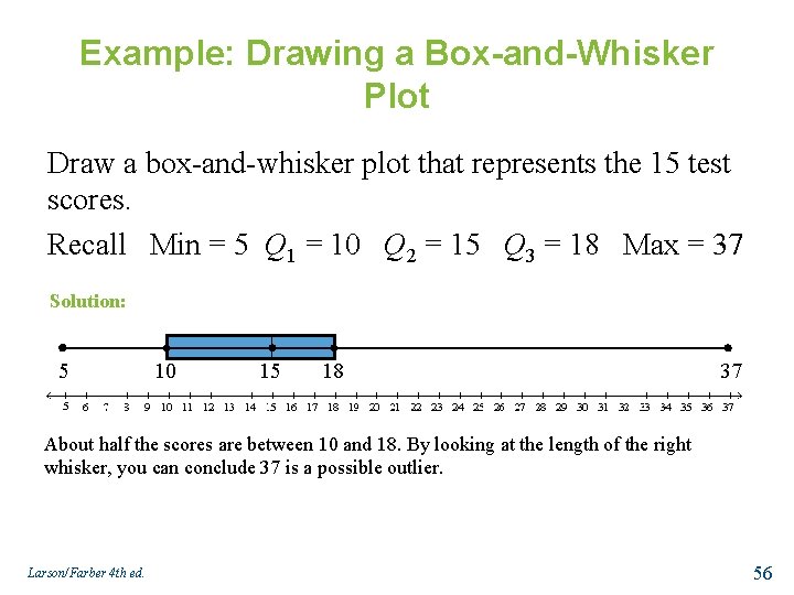
Example: Drawing a Box-and-Whisker Plot Draw a box-and-whisker plot that represents the 15 test scores. Recall Min = 5 Q 1 = 10 Q 2 = 15 Q 3 = 18 Max = 37 Solution: 5 10 15 18 37 About half the scores are between 10 and 18. By looking at the length of the right whisker, you can conclude 37 is a possible outlier. Larson/Farber 4 th ed. 56

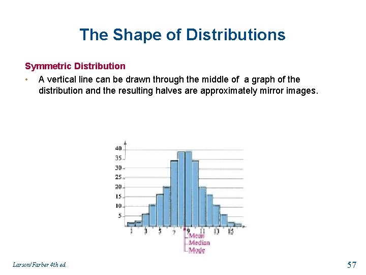
The Shape of Distributions Symmetric Distribution • A vertical line can be drawn through the middle of a graph of the distribution and the resulting halves are approximately mirror images. Larson/Farber 4 th ed. 57

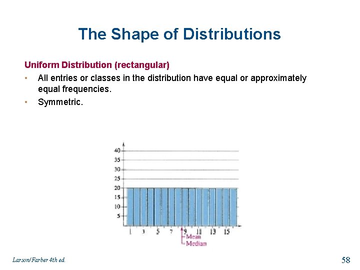
The Shape of Distributions Uniform Distribution (rectangular) • All entries or classes in the distribution have equal or approximately equal frequencies. • Symmetric. Larson/Farber 4 th ed. 58

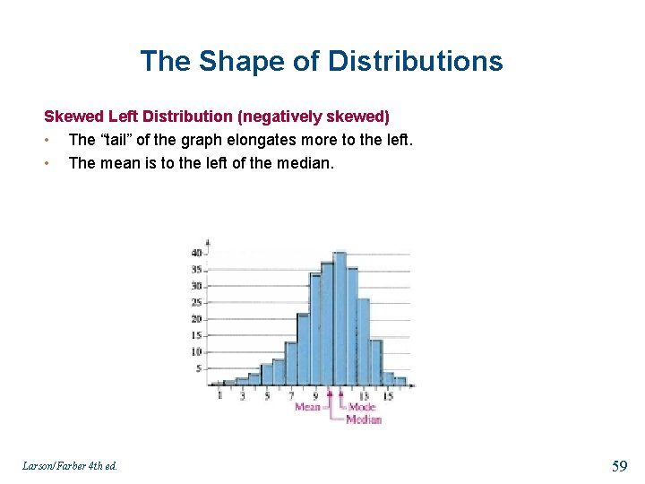
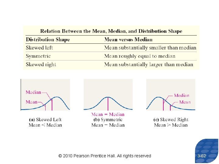
The Shape of Distributions Skewed Left Distribution (negatively skewed) • The “tail” of the graph elongates more to the left. • The mean is to the left of the median. Larson/Farber 4 th ed. 59

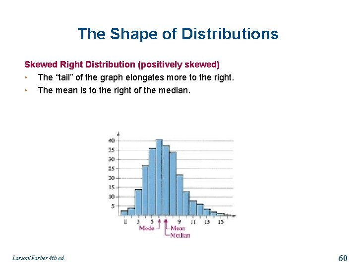
The Shape of Distributions Skewed Right Distribution (positively skewed) • The “tail” of the graph elongates more to the right. • The mean is to the right of the median. Larson/Farber 4 th ed. 60

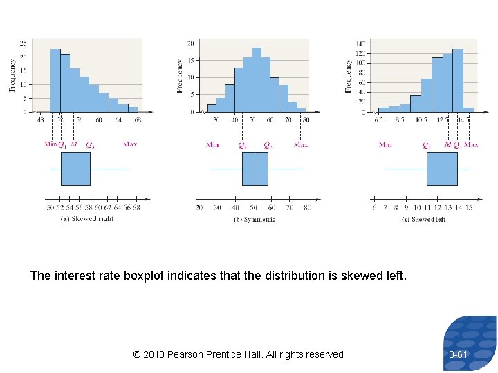
The interest rate boxplot indicates that the distribution is skewed left. © 2010 Pearson Prentice Hall. All rights reserved 3 -61

© 2010 Pearson Prentice Hall. All rights reserved 3 -62