What is JPEG 2000 JPEG 2000 is a

What is JPEG 2000? • JPEG 2000 is a new compression standard for still images intended to overcome the shortcomings of the existing JPEG standard. • The standardization process is coordinated by the Joint Technical Committee on Information technology of the International Organization for Standardization (ISO)/ International Electrotechnical Commission (IEC). • JPEG 2000 makes use of the wavelet and sub-band technologies. Some of the markets targeted by the JPEG 2000 standard are Internet, printing, digital photography, remote sensing, mobile, digital libraries and E-commerce. • The core compression algorithm is primarily based on the Embedded Block Coding with Optimized Truncation (EBCOT) of the bit-stream. The EBCOT algorithm provides a superior compression performance and produces a bitstream with features such as resolution and SNR scalability and random access. © V. Sanchez & A. Basu, University of Alberta

Features of JPEG 2000 ); ; Lossless and lossy compression: the standard provides lossy compression with a superior performance at low bit-rates. It also provides lossless compression with progressive decoding. Applications such as digital libraries/databases and medical imagery can benefit from this feature. ); ; Protective image security: the open architecture of the JPEG 2000 standard makes easy the use of protection techniques of digital images such as watermarking, labeling, stamping or encryption ); ; Region-of-interest coding: in this mode, regions of interest (ROI’s) can be defined. These ROI’s can be encoded and transmitted with better quality than the rest of the image. ); ; Robustness to bit errors: the standard incorporate a set of error resilient tools to make the bit-stream more robust to transmission errors. © V. Sanchez & A. Basu, University of Alberta

Features of JPEG 2000 (cont’d) Example of region of interest coding. A region of interest in the Barbara image is reconstructed with quality scalability. The region of interest is decoded first before any background information. Region of interest © V. Sanchez & A. Basu, University of Alberta

The JPEG 2000 Compression Engine Source Image Data Encoder Preprocessing Forward Transform Quantization Entropy Encoding Bit stream Storage or transmission Inverse Transform Reconstructed Image Data Inverse Quantization Entropy Decoding Decoder © V. Sanchez & A. Basu, University of Alberta Bit stream

Pre-processing Three steps: 1. Image tiling (optional)-7 for each image component. DWT on Each Tile Tiling DC Level Component Shifting Transformati on Image Component • DC level shifting -7 samples of each tile are subtracted the same quantity (i. e. component depth). • Color transformation (optional) -7 from RGB to Y Cb Cr © V. Sanchez & A. Basu, University of Alberta

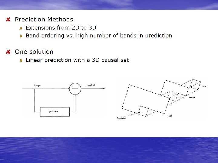
Forward Transform • Discrete Wavelet Transform (DWT) is used to decompose each tile component into different sub-bands. • The transform is in the form of dyadic decomposition and use biorthogonal wavelets. © V. Sanchez & A. Basu, University of Alberta

Forward Transform (cont’d) • DWT can be irreversible or reversible. ); ; Irreversible transform -7 Daubechies 9 -tap/7 -tap filter ); ; Reversible transform -7 Le Gall 5 -tap/3 -tap filter • Two filtering modes are supported: ); ; Convolution based ); ; Lifting based © V. Sanchez & A. Basu, University of Alberta

Analysis and Synthesis Filter Coefficients Le Gall 5/3 © V. Sanchez & A. Basu, University of Alberta

Analysis and Synthesis Filter Coefficients Daubchines 9/7 © V. Sanchez & A. Basu, University of Alberta

2 D-Forward Transform • 1 -D sets of samples are decomposed into low-pass and high-pass samples. • Low-pass samples represent a down-sampled, low resolution version of the original set. • High pass samples represent a down-sampled residual version of the original set (details). Low frequency information High frequency information (vertical details) High frequency information (horizontal details) High frequency information (diagonal details) © V. Sanchez & A. Basu, University of Alberta

© V. Sanchez & A. Basu, University of Alberta

Quantization • After transformation, all coefficients are quantized using scalar quatization. • Quantization reduces coefficients in precision. The operation is lossy unless the quatization step is 1 and the coefficients integers (e. g. reversible integer 5/3 wavelet). • The process follows the formula: a� b (u, v) � q b (u , v) sign (a b (u , v)) � � � b � Largest integer not exceeding ab Quantized value Transform coefficient of sub-band b Quantization step © V. Sanchez & A. Basu, University of Alberta

Modes of Quantization • Two modes of operation: ); ; Integer mode-7 integer-to-integer transforms are employed. Quantization step are fixed to one. Lossy coding is still achieved by discarding bit-planes. ); ; Real mode-7 real-to-real transforms are employed. Quantization steps are chosen in conjunction with rate control. In this mode, lossy compression is achieved by discarding bi-planes or changing the size of the quantization step or both. © V. Sanchez & A. Basu, University of Alberta

Code-blocks, precincts and packets 1 2 3 4 Precinct: each sub-band is divided into rectangular blocks called precincts. Packets: three spatially consistent rectangles comprise a packet. 5 6 9 10 7 8 11 12 Code-block: each precinct is further divided into non-overlapping rectangles called code-blocks. Each code-block forms the input to the entropy encoder and is encoded independently. Packet Code-block Precinct Sub-band Within a packet, code-blocks are visited in raster order. © V. Sanchez & A. Basu, University of Alberta

Entropy Coding: Bit-planes • The coefficients in a code block are separated into bit-planes. The individual bit-planes are coded in 1 -3 coding passes. Code-block 15 3 6 MSB Bit-plane representation 11 LSB 15 1 1 6 0 1 1 0 3 0 0 1 1 11 1 0 1 1 Coding passes Encoded data Bit-plane context based arithmetic coder © V. Sanchez & A. Basu, University of Alberta

Entropy Coding: Coding Passes • Each of these coding passes collects contextual information about the bit- plane data. The contextual information along with the bit-planes are used by the arithmetic encoder to generate the compressed bit-stream. • The coding passes are: ); ; Significance propagation pass -7 coefficients that are insignificant and have a certain preferred neighborhood are coded. ); ; Magnitude refinement pass -7 the current bits of significant coefficients are coded. ); ; Clean-up pass -7 the remaining insignificant coefficients for which no information has yet been coded are coded. © V. Sanchez & A. Basu, University of Alberta

JPEG 2000 Bit-stream • For each code-block, a separate bit-stream is generated. • The coded data of each code-block is included in a packet. • If more that one layer is used to encode the image information, the code-block bit-streams are distributed across different packets corresponding to different layers. H JPEG 2000 bit-stream Layer Main Header H Packet Header Packet Coded code-block © V. Sanchez & A. Basu, University of Alberta

How to tell if 2 Images are same? Pixel by pixel comparison? Makes sense only if pictures taken from same angle, same lighting, etc Noise, quantization, etc introduces differences Human may say images are same even with numerical differences

Comparing Images Better approach: Template matching Identify similar sub‐images (called template) within 2 images Applications? Match left and right picture of stereo images Find particular pattern in scene Track moving pattern through image sequence

Template Matching Basic idea Move given pattern (template) over search image Measure difference between template and sub‐images at different positions Record positions where highest similarity is found Sub. Image Template

Template Matching Difficult issues? What is distance (difference) measure? What levels of difference should be considered a match? How are results affected when brightness or contrast changes? Sub. Image Template

Template Matching in Intensity Images Consider problem of finding a template (reference image) R within a search image Can be restated as Finding positions in which contents of R are most similar to the corresponding subimage of I If we denote R shifted by some distance (r, s) by

Template Matching in Intensity Images We can restate template matching problem as: Finding the offset (r, s) such that the similarity between the shifted reference image Rr, s and corresponding subimage I is a maximum Solving this problem involves solving many sub‐problems

Distance between Image Patterns Many measures proposed to compute distance between the shifted reference image Rr, s and corresponding subimage I

Distance between Image Patterns Many measures proposed to compute distance between the shifted reference image Rr, s and corresponding subimage I Sum of absolute differences: Maximum difference: Sum of squared differences (also called N‐dimensional Euclidean distance):

Distance and Correlation Best matching position between shifted reference image Rr, s and subimage I minimizes square of d. E which can be expanded as B term is a constant, independent of r, s and can be ignored A term is sum of squared values within subimage I at current offset r, s

Distance and Correlation C(r, s) term is linear cross correlation between I and R defined as Since R and I are assumed to be zero outside their boundaries Note: Correlation is similar to linear convolution Min value of d 2 E(r, s) corresponds to max value of

Normalized Cross Correlation Unfortunately, A term is not constant in most images Thus cross correlation result varies with intensity changes in image I Normalized cross correlation considers energy in I and R CN (r, s) is a local distance measure, is in [0, 1] range CN (r, s) = 1 indicates maximum match CN (r, s) = 0 indicates images are very dissimilar

Correlation Coefficient Correlation coefficient: Use differences between I and R and their average values where the average values are defined as K is number of pixels in reference image R CL(r, s) can be rewritten as

Correlation Coefficient Algorithm

Correlation Coefficient Java Implementation

Correlation Coefficient Java Implementation

Examples and Discussion We now compare these distance metrics Original image I: Repetitive flower pattern Reference image R: one instance of repetitive pattern extracted from I Now compute various distance measures for this I and R

Examples and Discussion Sum of absolute differences: performs okay but affected by global intensity changes Maximum difference: Responds more to lighting intensity changes than pattern similarity

Examples and Discussion Sum of squared (euclidean) distances: performs okay but affected by global intensity changes Global cross correlation: Local maxima at true template position, but is dominated by high‐intensity responses in brighter image parts

Examples and Discussion Normalized cross correlation: results similar to euclidean distance (affected by global intensity changes) Correlation coefficient: yields best results. Distinct peaks produced for all 6 template instances, unaffected by lighting

Effects of Changing Intensity To explore effects of globally changing intensity, raise intensiy of reference image R by 50 units Distinct peaks disappear in Euclidean distance Correlation coefficient unchanged, robust measure in realistic lighting conditions

Euclidean Distance under Global Intensity Changes Distance function for original template R Distance function with intensity increased by 25 units Distance function with intensity increased by 50 units Local peaks disappear as template intensity (and thus distance) is increased

Shape of Template does not have to be rectangular Some applications use circular, elliptical or custom‐shaped templates Non‐rectangular templates stored in rectangular array, but pixels in template marked using a mask More generally, a weighted function can be applied to template elements

Matching under Rotation and Scaling Simple Approach: Store multiple rotated and scaled versions of template Computationally prohibitive Alternate approaches: Matching in logarithmic‐polar space (complicated!) Affine matching use local statistical features invariant under affine image transformations (including rotation and scaling)

Matching Binary Images Direct Comparison: Count the number of identical pixels in search image and template Small total difference when most pixels are same Problem: Small shift, rotation or distortion of image create high distance Need a more tolerant measure

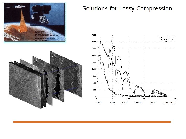
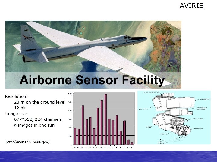
- 17 Mbps data rate through 1994, 20. 4 Mbps from 1995 to 2004, 16 bit from 2005 onward - 10 bit data encoding through 1994, 12 bit from 1995 - Silicon (Si) detectors for the visible range, indium gallium arsenide (In. Ga. Ar) for the NIR, and indiumantimonide (In. Sb) detectors for the SWIR - "Whisk broom" scanning - 12 Hz scanning rate - Liquid Nitrogen (LN 2) cooled detectors - 10 nm nominal channel bandwidth, calibrated to within 1 nm - 34 degrees total field of view (full 677 samples) - 1 milliradian Instantaneous Field Of View (IFOV, one sample), calibrated to within 0. 1 mrad - 76 GB hard disk recording medium

Introduction --Classification Shape Contour Structural Syntactic Graph Tree Model-driven Data-driven Region Non-Structural Perimeter Compactness Eccentricity Fourier Descriptors Wavelet Descriptors Curvature Scale Space Shape Signature Chain Code Hausdorff Distance Elastic Matching Area Euler Number Eccentricity Geometric Moments Zernike Moments Pseudo-Zernike Mmts Legendre Moments Grid Method

Boundary Descriptors • There are several simple geometric measures that can be useful for describing a boundary. – The length of a boundary: the number of pixels along a boundary gives a rough approximation of its length. – Curvature: the rate of change of slope • To measure a curvature accurately at a point in a digital boundary is difficult • The difference between the slops of adjacent boundary segments is used as a descriptor of curvature at the point of intersection of segments

Representation Skeletons • Skeletons: produce a one pixel wide graph that has the same basic shape of the region, like a stick figure of a human. It can be used to analyze the geometric structure of a region which has bumps and “arms”.

Representation Skeletons: Example • One application of • skeletonization is for character recognition. A letter or character is determined by the center-line of its strokes, and is unrelated to the width of the stroke lines.

Regional Descriptors Topological property 1: the number of holes (H) Topological property 2: the number of connected components (C)

Regional Descriptors Topological property 3: Euler number: the number of connected components subtract the number of holes E=C-H E=0 E= -1

Regional Descriptors Topological property 4: the largest connected component.

Regional Descriptors Texture

Regional Descriptors Texture • Texture is usually defined as the smoothness or • • roughness of a surface. In computer vision, it is the visual appearance of the uniformity or lack of uniformity of brightness and color. There are two types of texture: random and regular. – Random texture cannot be exactly described by words or equations; it must be described statistically. The surface of a pile of dirt or rocks of many sizes would be random. – Regular texture can be described by words or equations or repeating pattern primitives. Clothes are frequently made with regularly repeating patterns. – Random texture is analyzed by statistical methods. – Regular texture is analyzed by structural or spectral (Fourier) methods.

Regional Descriptors Statistical Approaches • Let z be a random variable denoting gray levels and let p(zi), i=0, 1, …, L-1, be the corresponding histogram, where L is the number of distinct gray levels. – The nth moment of z: – The measure R: – The uniformity: – The average entropy:

Regional Descriptors Statistical Approaches Smooth Coarse Regular

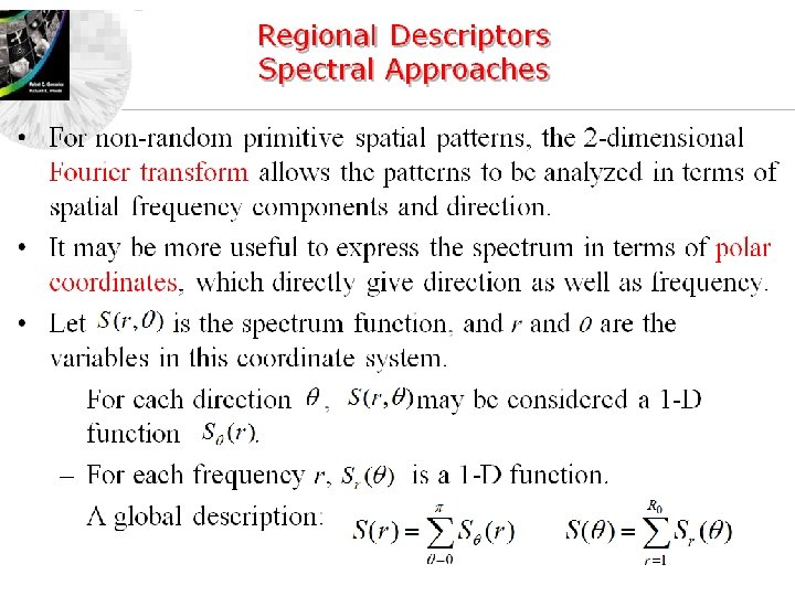
Regional Descriptors Spectral Approaches

Regional Descriptors Spectral Approaches

Regional Descriptors Moments of Two-Dimensional Functions • For a 2 -D continuous function f(x, y), the moment of order (p+q) is defined as • The central moments are defined as

Regional Descriptors Moments of Two-Dimensional Functions • If f(x, y) is a digital image, then • The central moments of order up to 3 are

Regional Descriptors Moments of Two-Dimensional Functions • The central moments of order up to 3 are

Regional Descriptors Moments of Two-Dimensional Functions • The normalized central moments are defined as

Regional Descriptors Moments of Two-Dimensional Functions • A seven invariant moments can be derived from the second and third moments:

Regional Descriptors Moments of Two-Dimensional Functions • • This set of moments is invariant to translation, rotation, and scale change.

Regional Descriptors Moments of Two-Dimensional Functions

Regional Descriptors Moments of Two-Dimensional Functions Table 11. 3 Moment invariants for the images in Figs. 11. 25(a)-(e).

The End