What is it all about How to use

What is it all about ? • How to use graphs to represent probability distributions over thousands of random variables ? • How to encode conditional independence in directed and undirected graphs ? • How to use such representations for efficient computations of the probability of events of interest ? • How to learn such models from data ? 2

Course Information Meetings: · Lecture: Mondays 10: 30 – 12: 30 · Tutorial: Mondays 13: 30 – 14: 30 Grade: u 40% in 4 question sets. These questions sets are obligatory. Each contains mostly theoretical problems. Submit in pairs before due time (three weeks). u 50% Bochan on January 9, based on first 9 weeks including Chanuka, and on understanding Chapter 3 & 4 of Pearl’s book. Obligatory to PASS the test and get a grade, but grade is fully replaceable with a programming project using BNs software. Miluim has to send me an advanced notice two weeks before the Bochan. u 10%. Obligatory for a **passing grade**. Attending all lectures and recitation classes except one. (In very special circumstances 2% per missing lecture or recitation). u u Prerequisites: Data structure 1 (cs 234218) Algorithms 1 (cs 234247) Probability (any course) Information and handouts: u http: //webcourse. cs. technion. ac. il/236372 u http: //www. cs. technion. ac. il/~dang/course. BN/ (Only lecture slides) 3

Relations to Some Other Courses. אמור לי מי חבריך ואומר לך מי אתה u Introduction to Artificial Intelligence (cs 236501) u Introduction to Machine Learning (cs 236756) u Introduction to Neural Networks (cs 236950) u Algorithms in Computational Biology (cs 236522) u Error correcting codes u Data mining u Vision 4

u u Mathematical Foundations Inference with Bayesian Networks Learning Bayesian Networks Applications 5

Homework • HMW #1. Read Chapter 3. 1 & 3. 2. 1. Answer Questions 3. 1, 3. 2, Prove Eq 3. 5 b, and fully expand the proof details of Theorem 2. Submit in pairs no later than noon of 14/11/16 (Two weeks). Pearl’s book contains all the notations that I happen not to define in these slides – consult it often – it is also a very unique and interesting classic text book. 6

The Traditional View of Probability in Text Books • Probability theory provides the impression that we need to literally represent a joint distribution explicitly as P(x 1, …, xn) on all propositions and their combinations. It is consistent and exhaustive. • This representation stands in sharp contrast to human reasoning: It requires exponential computations to compute marginal probabilities like P(x 1) or conditionals like P(x 1|x 2). • Humans judge pairwise conditionals swiftly while conjunctions are judged hesitantly. Numerical calculations do not reflect simple reasoning tasks. 7

The Qualitative Notion of Dependence • Marginal independence is defined numerically as P(x, y)=P(x) P(y). The truth of this equation is hard to judge by humans, while judging whether X and Y are dependent is often easy. • “Burglary within a day” and “nuclear within five years” • Likewise, the three place relationship (X influences Y, given Z) is judjed easily. For example: X = time of last pickup from a bus station and Y= time for next bus are dependent, but are conditionally independent given Z= whereabouts of the next bus 8

• The notions of relevance and dependence are far more basic than the numerical values. In a resonating system it should be asserted once and not be sensitive to numerical changes. • Acquisition of new facts may destroy existing dependencies as well as creating new once. • Learning child’s age Z destroys the dependency between height X and reading ability Y. • Learning symptoms Z of a patient creates dependencies between the diseases X and Y that could account for it. Probability theory provides in principle such a device via P(X | Y, K) = P(X |K) But can we model the dynamics of dependency changes based on logic, without reference to numerical quantities ? 9

Definition of Marginal Independence Definition: IP(X, Y) iff for all x DX and y Dy Pr(X=x, Y=y) = Pr(X=x) Pr(Y=y) Comments: u Each Variable X has a domain DX with value (or state) x in DX. u We often abbreviate via P(x, y) = P(x) P(y). u When Y is the emptyset, we get Pr(X=x) = Pr(X=x). u Alternative notations to IP(X, Y) such as: I(X, Y) or X Y u Next few slides on properties of marginal independence are based on “Axioms and algorithms for inferences involving probabilistic independence. ” 10

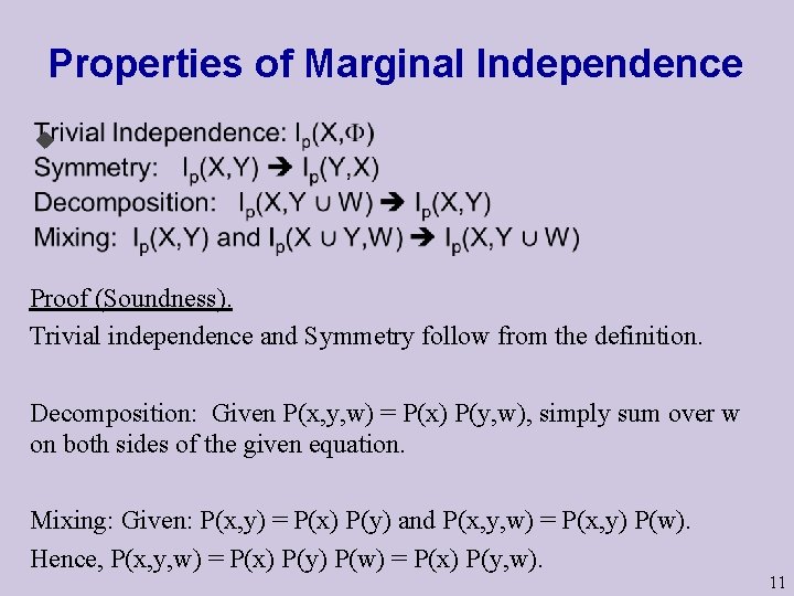
Properties of Marginal Independence u Proof (Soundness). Trivial independence and Symmetry follow from the definition. Decomposition: Given P(x, y, w) = P(x) P(y, w), simply sum over w on both sides of the given equation. Mixing: Given: P(x, y) = P(x) P(y) and P(x, y, w) = P(x, y) P(w). Hence, P(x, y, w) = P(x) P(y) P(w) = P(x) P(y, w). 11

Properties of Marginal Independence Are there more such independent properties of independence ? No. There are none ! 1. No more independent axioms of the form 1 & … & n where each statement stands for an independence statement. 2. We use the symbol for a set of independence statements. In this notation: is derivable from via these properties if and only if is entailed by (i. e. , holds in all probability distributions that satisfy ). 3. For every set and a statement not derivable from , there exists a probability distribution P that satisfies and not . 12

Properties of Marginal Independence Can we use these properties to infer a new independence statements from a set of given independence statements in polynomial time ? YES. The “membership algorithm” and completeness proof in Recitation class today (Paper P 2). Comment. The question “does entail ” could in principle be undecidable, drops to being decidable via a complete set of axioms, and then drops to polynomial with the above claim. 13

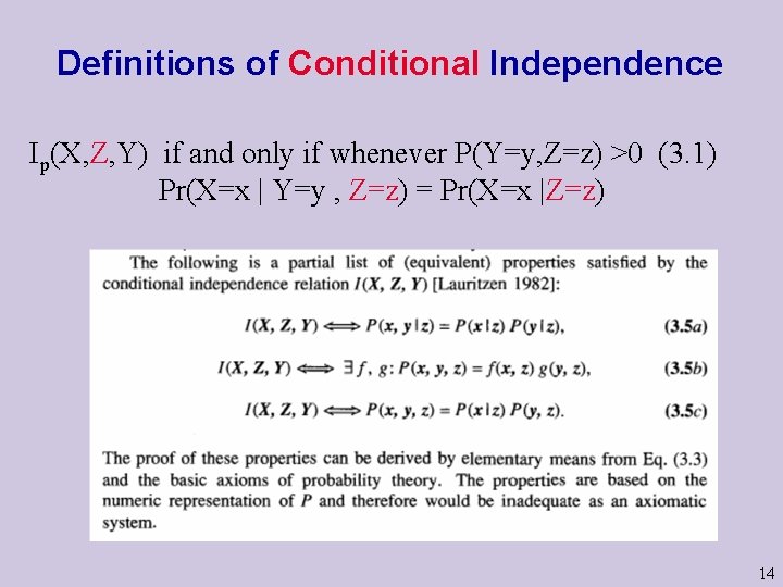
Definitions of Conditional Independence Ip(X, Z, Y) if and only if whenever P(Y=y, Z=z) >0 (3. 1) Pr(X=x | Y=y , Z=z) = Pr(X=x |Z=z) 14

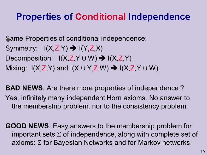
Properties of Conditional Independence u 15

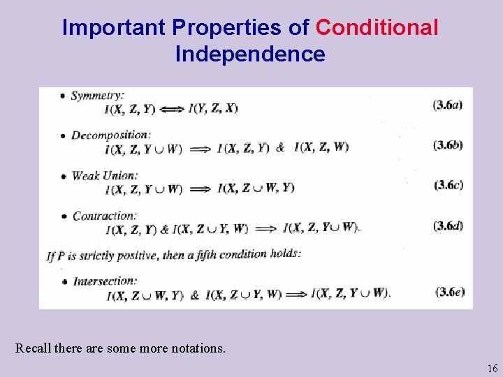
Important Properties of Conditional Independence Recall there are some more notations. 16

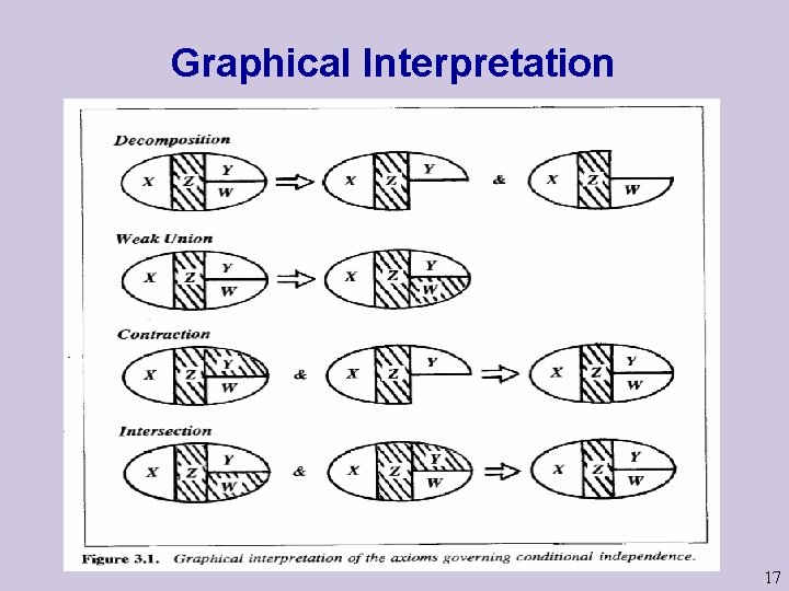
Graphical Interpretation 17

Use graphs and not pure logic • Variables represented by nodes and dependencies by edges. • Common in our language: “threads of thoughts”, “lines of reasoning”, “connected ideas”, “far-fetched arguments”. • Still, capturing the essence of dependence is not an easy task. When modeling causation, association, and relevance, it is hard to distinguish between direct and indirect neighbors. • If we just connect “dependent variables” we will get cliques. 18

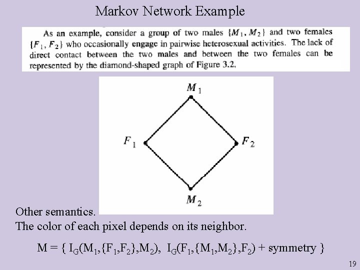
Markov Network Example Other semantics. The color of each pixel depends on its neighbor. M = { IG(M 1, {F 1, F 2}, M 2), IG(F 1, {M 1, M 2}, F 2) + symmetry } 19

Markov Networks 1. Define for each (maximal) clique Ci a nonnegative function g(Ci) called the compatibility function. 2. Take the product i g(Ci) over all cliques. 3. Define P(X 1, …, Xn) = K· i g(Ci) where K is a normalizing factor (inverse sum of the product). Mp = { IP(M 1, {F 1, F 2}, M 2), IP(F 1, {M 1, M 2}, F 2) + symmetry } SOUNDNESS: IG(X, Z, Y) IP(X, Z, Y) For all, sets of nodes X, Y, Z 20

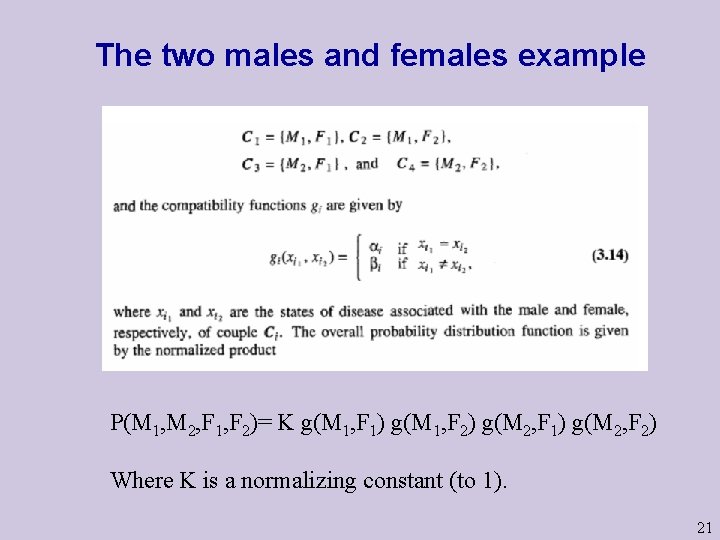
The two males and females example P(M 1, M 2, F 1, F 2)= K g(M 1, F 1) g(M 1, F 2) g(M 2, F 1) g(M 2, F 2) Where K is a normalizing constant (to 1). 21

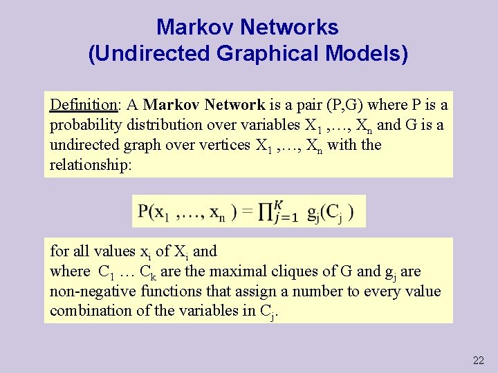
Markov Networks (Undirected Graphical Models) Definition: A Markov Network is a pair (P, G) where P is a probability distribution over variables X 1 , …, Xn and G is a undirected graph over vertices X 1 , …, Xn with the relationship: for all values xi of Xi and where C 1 … Ck are the maximal cliques of G and gj are non-negative functions that assign a number to every value combination of the variables in Cj. 22

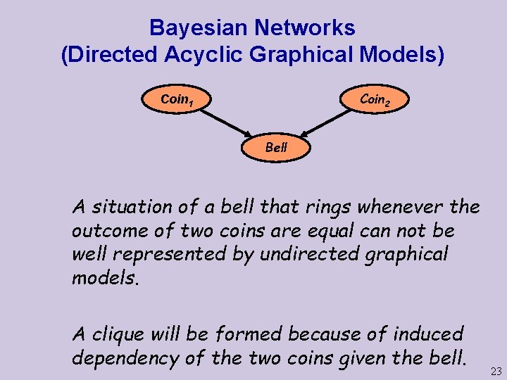
Bayesian Networks (Directed Acyclic Graphical Models) Coin 2 Coin 1 Bell A situation of a bell that rings whenever the outcome of two coins are equal can not be well represented by undirected graphical models. A clique will be formed because of induced dependency of the two coins given the bell. 23

Bayesian Networks (BNs) Examples of models for diseases & symptoms & risk factors One variable for all diseases (values are diseases) One variable per disease (values are True/False) Naïve Bayesian Networks versus Bipartite BNs 24

Natural Direction of Information Even simple tasks are not natural to phrase in terms of joint distributions. Consider the example of a hypothesis H=h indicating a rare disease and A set of symptoms such as fever, blood preasure, pain, etc, marked by E 1=e 1, E 2=e 2, E 3=e 3 or in short E=e. We need P(h | e). Can we naturally assume P(H, E) is given and compute P(h | e) ? 25