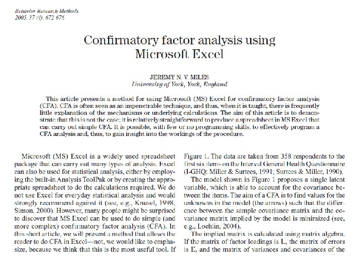
What is applied psychometrics Tim Croudace tjc 39cam


 • Announcement about summer schools • Announcement")


")


. The statistics of")

 psychometry Etymologically (from the Greek) - psychometry means - measuring the")


![What is ? [Psychometric] Test Theory • Psychometric Test Theory …is essentially a collection](https://slidetodoc.com/presentation_image_h/996beefcb19e489af174d52f0055bb6b/image-17.jpg "What is ? [Psychometric] Test Theory • Psychometric Test Theory …is essentially a collection")
 Item Response Modelling (IRM) IRT refers to")
 Theory : 2 main schools, old & new Classical Test Theory Item")


: STATA factor command factor v 1 -v 8, factors(2) ml")
 Exploratory Factor Analysis (ML): STATA rotate command. rotate, bentler bl(. 35) Rotated factor")
: STATA cfa 1 command Log likelihood = -457. 31642 |")
: STATA confa commands. confa (f: v 1 -v 8), from(2")
: STATA estat fitindices commands Fit indices RMSEA = 0. 2276")
: STATA confa command (2 factors) confa (f 1: v 1")
: STATA confa commands. estat fitindices Fit indices RMSEA RMSR TLI")
")


 is")

 (1 random effect (individual differences – x – axis))")


 location")
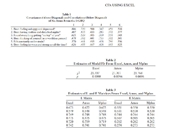
![parscale ITEM FIT STATISTICS [not to be trusted for short tests, illustrative only] |](https://slidetodoc.com/presentation_image_h/996beefcb19e489af174d52f0055bb6b/image-43.jpg "parscale ITEM FIT STATISTICS [not to be trusted for short tests, illustrative only] |")
 Y-axis conditional standard error of measurement")

 Non-parametric IRT Mokken Analysis STATA msp command. msp GHQ 1 -GHQ 12, c(.")
 Non-parametric IRT Mokken Analysis STATA msp command Scale: 2 -----Significance level: 0. 016667")
 Rasch model in STATA Estimation method: Conditional maximum likelihood (CML) Number of items:")
 Rasch model in STATA raschtest Ability Expected Group Score parameters std Err. Freq.")


 Author: Ivailo Partchev <Ivailo. Partchev@uni-jena. de>")
 • • • The")
 Extract from //cran. r-project. org/web/views/Psychometrics. html Item Response Theory (IRT): • The e.")
 Extract from //cran. r-project. org/web/views/Psychometrics. html Structural Equation Models, Factor Analysis, PCA: •")


 Application oriented book • see Chapter by Assessing Quality of")


- Slides: 74
What is applied psychometrics? Tim Croudace tjc 39@cam. ac. uk Department of Psychiatry John Rust jnr 24@cam. ac. uk The Psychometrics Centre University of Cambridge
What is applied psychometrics? Professor John Rust http: //www. ppsis. psychometrics. cam. ac. uk
Overview • • • About the Centre What is psychometrics? Psychometrics today What we are doing now What we are going to do
The Psychometric Centre • • • Educational and diagnostic eg Wechsler Organisational eg Watson-Glaser, Orpheus Statistical, IRT and AI techniques Computer languages eg Mplus, Stata, R Web based assessment BPS Level A and B courses Seminars, workshops and summer schools Ph. Ds in psychometrics or related areas Tutorial materials on website – www. psychometrics. ppsis. cam. ac. uk 4
Current activities • Who we are (people) • Announcement about summer schools • Announcement about forthcoming workshops
What is psychometrics? • “The science of psychological assessment” • Much assessment is “high stakes” • • Questionnaires and social surveys Recruitment and staff development Licensing and chartering (eg Accountants, Surgeons) School and University examinations Psychiatric and ‘special needs’ diagnosis Credit ratings Career guidance Social awareness
Types of assessment • • First impressions Application forms and references Objective tests (on or off line) Projective tests Interviews Essays and examinations Research questionnaires and semi-structured interviews 7
The Psychometric Principles Maximizing the quality of assessment • • Reliability (freedom from error) Validity ( ‘. . . what is says on the tin’) Standardisation (compared with what? ) Equivalence (is it biased? ) • Rust, J. & Golombok, S. (2009) Modern Psychometrics • (3 rd Edition): Taylor and Francis: London 8
Can everything be measured? • “If anything exists it must exist in some quantity and can therefore be measured”. (Lord Kelvin 1824, 1907) • In 1900, Lord Kelvin claimed "There is nothing new to be discovered in physics now. All that remains is more and more precise measurement. "[ 9
The theory of true scores • Whatever precautions have been taken to secure unity of standard, there will occur a certain divergence between the verdicts of competent examiners. • If we tabulate the marks given by the different examiners they will tend to be disposed after the fashion of a gendarme’s hat. • I think it is intelligible to speak of the mean judgment of competent critics as the true judgment; and deviations from that mean as errors. • This central figure which is, or may be supposed to be, assigned by the greatest number of equally competent judges, is to be regarded as the true value . . . , just as the true weight of a body is determined by taking the mean of several discrepant measurements. • Edgeworth, F. Y. (1888). The statistics of examinations. Journal of the Royal Statistical Society, LI, 599 -635. 10
The evolution of the Latent Trait • Edgeworth, F. Y. (1888). The statistics of examinations. Journal of the Royal Statistical Society, LI, 599 -635. With two measures of the same characteristic we can estimate true values. • Melvin Novik and Frederick Lord (1968) “Statistical theories of mental test scores” use Classical Test Theory to derive Latent Trait Theory. Allan Birnbaum, in his supplement, established Item Response Theory of which Rasch Scaling is a special case. • Today Latent Variable Analysis (LVA) is an integral part of statistical modelling in Psychometrics, Econometrics and Statistics. 11
What is applied psychometrics? Tim Croudace tjc 39@cam. ac. uk Department of Psychiatry University of Cambridge
psycho·met·rics (sī′kō me′triks) psychometry Etymologically (from the Greek) - psychometry means - measuring the mind P. Kline (1979) “The meaning of psychometrics” p 1
-definitions-definitions • Collins English Dictionary Psychometrics definition : psychometrics n 1. the branch of psychology concerned with the design and use of psychological tests 2. application of statistical & mathematical techniques to psychological testing • dictionary. reverso. net/englishdefinition/psychometrics
What is psychometrics? The Science of Psychological Assessment “the branch of psychology dealing with measurable factors” Modern Psychometrics. by J. Rust & S. Golombok. Routledge. P 4
Even Wikipedia has something to say … it doesn’t begin too promisingly!!! [From Wikipedia, the free encyclopedia] Psychometrics – Not to be confused with psychrometrics, the measurement of the heat and water vapor properties of air. For other uses of this term and similar terms, see (disambiguation). Psychometry [Redirected from Psychometry (disambiguation)] may refer to: Psychometry (paranormal) a form of extrasensory perception Psychometrics a discipline of psychology and education (getting warmer!!) And finally it begins to make sense … – Psychometrics is the field of study concerned with theory and technique of educational and psychological measurement, which includes the measurement of knowledge, abilities, attitudes, and personality traits. The field is primarily concerned with the construction and validation of measurement instruments, such as questionnaires, tests, and personality assessments.
What is ? [Psychometric] Test Theory • Psychometric Test Theory …is essentially a collection of mathematical concepts that formalize and clarify certain questions about constructing and using tests [and scales] and then provide methods for answering them R. P. Mc. Donald (1999) Test Theory: a unified treatment. LEA. P 9
What is psychometrics? Item Response Theory (IRT) Item Response Modelling (IRM) IRT refers to a set of mathematical models that describe, in probabilistic terms, the relationship between a person’s response to a survey question/test item and his or her level of the ‘latent variable’ being measured by the scale Fayers and Hays p 55 – Assessing Quality of Life in Clinical Trials. Oxford Univ Press: – Chapter on Applying IRT for evaluating questionnaire item and scale properties.
Psychometric (Measurement) Theory : 2 main schools, old & new Classical Test Theory Item response theory • Associated with use of traditional (old) psychometric methods • Modern test theory • A set or family of mathematical / probability models that describe the relationship between a person’s [response / answer] to a [questionnaire survey / test item] and his or her level of the latent variable being measured – linear factor analysis – Cronbach’s alpha (internal consistency), – summing items and simple sum scores
Classical Test Theory Reliability estimation Reliability coefficient Major error source Data-gathering procedure Statistical data analysis 1. Stability coefficient Changes over time Test-retest Produce-moment correlation 2. Equivalence coefficient Item sampling: from test form to test form Produce-moment correlation 3. Internal consistency coefficient Item sampling: A single test heterogeneity administration Given form j, form k a) Split-half correlation/ Spearman Brown correction, b) coefficient alpha c) Factor loadings d) Other Table 4. 1 p 26 Dato M. N. De Gruiter and Leo J. Th. Van der Kamp (2008)
Reliability coefficients STATA alpha and cialpha commands Continuous outcomes: Guttman-Cronbach alpha Test scale = mean(unstandardized items) Average interitem covariance: Number of items in the scale: Scale reliability coefficient: . 0921364 8 0. 7942 Cronbach's alpha one-sided confidence interval ----------------------------------Items | alpha [95% Conf. Interval] -----+-----------------------------Test |. 79423639 >=. 7348227 -----------------------------------
Exploratory Factor Analysis (ML): STATA factor command factor v 1 -v 8, factors(2) ml Factor analysis/correlation Method: maximum likelihood Rotation: (unrotated) Number of obs = 87 Retained factors = 2 Number of params = 15 Schwarz's BIC = 95. 9898 Log likelihood = -14. 5006 (Akaike's) AIC = 59. 0012 -------------------------------------Factor | Eigenvalue Difference Proportion Cumulative -------+------------------------------Factor 1 | 2. 84462 1. 43839 0. 6692 Factor 2 | 1. 40624. 0. 3308 1. 0000 -------------------------------------LR test: independent vs. saturated: chi 2(28) = 261. 31 Prob>chi 2 = 0. 0000 LR test: 2 factors vs. saturated: chi 2(13) = 27. 39 Prob>chi 2 = 0. 0110 Factor loadings (pattern matrix) and unique variances Variable | Factor 1 Factor 2 | Uniqueness v 1 | 0. 6652 -0. 2760 | 0. 4814 v 2 | 0. 8126 -0. 2484 | 0. 2780 v 3 | 0. 7071 -0. 3337 | 0. 3886 v 4 | 0. 7123 -0. 0119 | 0. 4925 v 5 | 0. 4729 0. 4383 | 0. 5842 v 6 | 0. 3554 0. 6141 | 0. 4966 v 7 | 0. 3969 0. 5332 | 0. 5581 v 8 | 0. 4764 0. 5507 | 0. 4698 -------------------------
(2) Exploratory Factor Analysis (ML): STATA rotate command. rotate, bentler bl(. 35) Rotated factor loadings (pattern matrix) and unique variances Variable | Factor 1 Factor 2 | Uniqueness -------------+-------------v 1 | 0. 7188 | 0. 4814 v 2 | 0. 8392 | 0. 2780 v 3 | 0. 7819 | 0. 3886 v 4 | 0. 6452 | 0. 4925 v 5 | 0. 6015 | 0. 5842 v 6 | 0. 7078 | 0. 4966 v 7 | 0. 6533 | 0. 5581 v 8 | 0. 7039 | 0. 4698 ------------------------(blanks represent abs(loading)<. 35) Factor rotation matrix | Factor 1 Factor 2 -------+---------Factor 1 | 0. 8985 0. 4390 Factor 2 | -0. 4390 0. 8985 ----------------
Confirmatory Factor Analysis (ML): STATA cfa 1 command Log likelihood = -457. 31642 | Coef. Std. Err. z P>|z| Lambda | v 1 | 1. v 2 | 1. 146607. 1706831 v 3 | 1. 077999. 1776428 v 4 | 1. 128529. 1988093 v 5 |. 6362603. 2008189 v 6 |. 4119255. 2019811 v 7 |. 5417541. 2211306 v 8 |. 6653727. 2206966 Var[error] | v 1 |. 1172731. 0215309 v 2 |. 0669433. 0176594 v 3 |. 1085488. 0212332 v 4 |. 1349088. 0264226 v 5 |. 240713. 038299 v 6 |. 2753728. 0426118 v 7 |. 3244316. 0504165 v 8 |. 2991244. 0473675 Var[latent] | phi 1 |. 1107746. 0320436 Goodness of fit test: LR = 109. 116 ; Test vs independence: LR = 163. 149 ; Number of obs = 87 [95% Conf. Interval]. 6. 72 6. 07 5. 68 3. 17 2. 04 2. 45 3. 01 . 0. 000 0. 002 0. 041 0. 014 0. 003 . . 8120748. 729825. 7388694. 2426624. 0160498. 1083461. 2328152 . 1. 48114 1. 426172 1. 518188 1. 029858. 8078011. 975162 1. 09793 5. 45 3. 79 5. 11 6. 29 6. 46 6. 44 6. 31 0. 000 0. 000 . 0750732. 0323315. 0669325. 0831214. 1656483. 1918553. 225617. 2062859 . 159473. 1015551. 1501651. 1866963. 3157778. 3588903. 4232461. 391963 3. 46 0. 001. 0479702 Prob[chi 2(20) > LR] = 0. 0000 Prob[chi 2( 8) > LR] = 0. 0000 . 173579
Single factor model (ML): STATA confa commands. confa (f: v 1 -v 8), from(2 SLS) log likelihood = -457. 31642 | Coef. Std. Err. Loadings | f | v 1 | 1. v 2 | 1. 146608. 1706831 v 3 | 1. 077998. 1776429 v 4 | 1. 128529. 1988093 v 5 |. 6362603. 2008189 v 6 |. 4119255. 2019811 v 7 |. 5417541. 2211306 v 8 |. 6653728. 2206967 Var[error] | v 1 |. 1172731. 0215309 v 2 |. 0669433. 0176594 v 3 |. 1085489. 0212332 v 4 |. 1349088. 0264226 v 5 |. 2407129. 038299 v 6 |. 2753727. 0426117 v 7 |. 3244316. 0504165 v 8 |. 2991244. 0473675 Goodness of fit test: LR = 109. 116 Test vs independence: LR = 163. 149 z P>|z| Number of obs = 87 [95% Conf. Interval] . 6. 72 6. 07 5. 68 3. 17 2. 04 2. 45 3. 01 . 0. 000 0. 002 0. 041 0. 014 0. 003 . . 8120749. 7298248. 7388694. 2426625. 0160499. 1083461. 2328153 . 1. 48114 1. 426172 1. 518188 1. 029858. 8078012. 9751621 1. 09793 5. 45 3. 79 5. 11 6. 29 6. 46 6. 44 6. 31 0. 000 0. 000 . 0750732. 0323315. 0669326. 0831214. 1656482. 1918553. 2256171. 2062858 . 1594729. 1015551. 1501652. 1866962. 3157776. 3588902. 4232462. 3919629 ; Prob[chi 2(20) > LR] = 0. 0000 ; Prob[chi 2( 8) > LR] = 0. 0000
Confirmatory Factor Analysis (ML): STATA estat fitindices commands Fit indices RMSEA = 0. 2276 0. 2703) RMSR = 0. 0724 90% CI= (0. 1868, TLI CFI = 0. 7702 = 0. 2967 AIC BIC = = 946. 633 986. 087
Multidimensional factor model (ML): STATA confa command (2 factors) confa (f 1: v 1 -v 4) (f 2: v 5 -v 8), from(2 SLS) log likelihood = -422. 79486 Number of obs = 87 | Coef. Std. Err. z P>|z| [95% Conf. Interval] Means | v 1 | 1. 592161. 051198 31. 10 0. 000 1. 491814 1. 692507 v 2 | 1. 48841. 0494312 30. 11 0. 000 1. 391526 1. 585293 v 3 | 1. 568607. 0522239 30. 04 0. 000 1. 46625 1. 670964 v 4 | 1. 509285. 056323 26. 80 0. 000 1. 398894 1. 619677 v 5 | 1. 582903. 0572911 27. 63 0. 000 1. 470614 1. 695191 v 6 | 1. 511862. 0581486 26. 00 0. 000 1. 397893 1. 625831 v 7 | 1. 500861. 0640531 23. 43 0. 000 1. 37532 1. 626403 v 8 | 1. 456359. 0632607 23. 02 0. 000 1. 332371 1. 580348 Loadings | v 1 | 1. . . v 2 | 1. 129181. 1617634 6. 98 0. 000. 812131 1. 446232 v 3 | 1. 085591. 1685842 6. 44 0. 000. 7551719 1. 41601 v 4 | 1. 037635. 1794024 5. 78 0. 000. 6860131 1. 389258 v 5 | 1. . . v 6 | 1. 132231. 2299847 4. 92 0. 000. 6814688 1. 582992 v 7 | 1. 194321. 2745619 4. 35 0. 000. 6561897 1. 732453 v 8 | 1. 26779. 2739953 4. 63 0. 000. 7307694 1. 804811 Factor cov. | f 1 -f 1 |. 1190851. 0326402 3. 65 0. 000. 0551115. 1830586 f 2 -f 2 |. 1128016. 0399112 2. 83 0. 005. 0345771. 191026 f 1 -f 2 |. 040931. 017838 2. 29 0. 022. 0059692. 0758928 Goodness of fit test: LR = 40. 073 ; Prob[chi 2(19) > LR] = 0. 0032 Test vs independence: LR = 232. 192 ; Prob[chi 2( 9) > LR] = 0. 0000
Single factor model (ML): STATA confa commands. estat fitindices Fit indices RMSEA RMSR TLI CFI AIC BIC = = = 0. 1136, 90% CI= (0. 0637, 0. 1627) 0. 0299 0. 9553 0. 8205 879. 590 921. 510
Reliability coefficients STATA kr 20 command Kuder-Richardson KR 20 Kuder-Richarson coefficient of reliability (KR-20) Number of items in the scale = 12 Number of complete observations = 6299 Item-rest Item | Obs difficulty variance correlation -----+---------------------GHQ 1 | 6299 0. 1846 0. 1505 0. 4834 GHQ 2 | 6299 0. 1640 0. 1371 0. 3865 GHQ 3 | 6299 0. 1872 0. 1521 0. 1954 GHQ 4 | 6299 0. 1029 0. 0923 0. 4652 GHQ 5 | 6299 0. 1691 0. 1405 0. 4432 GHQ 6 | 6299 0. 0489 0. 0465 0. 3846 GHQ 7 | 6299 0. 1208 0. 1062 0. 5549 GHQ 8 | 6299 0. 1103 0. 0982 0. 5289 GHQ 9 | 6299 0. 0749 0. 0693 0. 3143 GHQ 10 | 6299 0. 0608 0. 0571 0. 3838 GHQ 11 | 6299 0. 1218 0. 1069 0. 4053 GHQ 12 | 6299 0. 1580 0. 1330 0. 5043 -----+---------------------Test | 0. 1253 0. 4208 KR 20 = 0. 7760
Reliability coefficients STATA kr 20 command Computes the reliability coefficient of a set of dichotomous items, [Cronbach's alpha is used for multipoint scales] In addition, kr 20 computes: - the item difficulty (proportion of 'right' answers), - the average value of item difficulty, - the item variance, - the corrected item-test point-biserial correlation coefficients, - the average value of corrected item-test correlation coefficients. The items must be coded as: - '0' for a wrong answer (unexpected answer), - '1' for a right answer (expected answer).
What is applied psychometrics? Tim Croudace tjc 39@cam. ac. uk Department of Psychiatry John Rust jnr 24@cam. ac. uk The Psychometrics Centre University of Cambridge
Message TRI IRT
Latent Trait Modelling Note: IRT = IRM = LTM = CDFA* • Latent trait modelling = factor analysis of categorical (binary/ordinal/nominal) data • Unidimensional LTM is widely used to measure variables/constructs such as • • • Personality Dimensions and Intelligence Ability: Mathematical / Verbal / Spatial Social and political attitudes Consumer preferences Health, Quality of life, Severity of disorder or symptoms e. g. in depression, back pain, fatigue etc… • Multidimensional IRT is statistically developed but is less widely used presently
Here the criterion 1 – 4 are binary but the latent variable (x-axis) is continuous (gaussian norm From Muthen, B. O (1991). Latent variable epidemiology. Alcohol Research World. 42 139 -167.
8 IRT models you might see …
Rasch model (logistic mixed model) (1 random effect (individual differences – x – axis)) 12 fixed effects – item thresholds (location of s-shapes along x) [Stata raschtest mixed effects logistic regression [inc gllamm] Item Discriminations GHQ 1 1. 095 GHQ 4 1. 095 GHQ 5 1. 095 GHQ 6 1. 095 GHQ 9 1. 095 GHQ 10 1. 095 GHQ 11 1. 095 GHQ 12 1. 095 GHQ 20 1. 095 GHQ 26 1. 095 Item Difficulties GHQ 1$1 GHQ 5$1 GHQ 12$1 GHQ 11$1 GHQ 26$1 GHQ 4$1 GHQ 20$1 GHQ 9$1 GHQ 10$1 GHQ 6$1 0. 021 0. 021 1. 226 1. 306 1. 364 1. 598 1. 601 0. 028 0. 029 0. 030 0. 033 1. 855 1. 986 2. 146 2. 283 0. 039 0. 045 0. 048
IRT in the Stata Journal J-7 -3 st 0129 . Est. dichotomous & ordinal item response models with gllamm By X. Zheng and S. Rabe-Hesketh Q 3/07 SJ 7(3): 313— 333 describes the one- and two-parameter logit models for dichotomous items the partial-credit and rating scale models for ordinal items, and an extension of these models where the latent variable is regressed on explanatory variables SJ-7 -1 st 0119 Rasch analysis: Estimation and tests with raschtest By J. Hardouin Q 1/07 SJ 7(1): 22 --44 command for estimating the Rasch model, the best known item response theory model for binary responses
Running Commercial IRT software from Stata runparscale: runparscale brings the IRT analysis framework of PARSCALE into the Stata enviroment. While runparscale does little more than data reformat and ascii file creation, it removes a lot of the hassle of estimating IRT models. Authors: runparscale was written by Laura Gibbons, Ph. D and Richard Jones, Sc. D, under the direction of Paul Crane, MD MPH. We appreciate the assistance of Tom Koepsell, MD MPH. Please see runparscale. ado for UW License information. Laura Gibbons, Ph. D gibbonsl@u. washington. edu Richard N Jones, Sc. D jones@mail. hrca. harvard. edu
Running Commercial IRT software from Stata runparscale
Running Commercial IRT software from Stata runparscale PARSCALE ITEM PARAMETERS item slope (se) location (se) -------------------------1 GHQ 1 1. 001 (0. 091) -0. 252 (0. 063) 2 GHQ 2 0. 433 (0. 060) 0. 170 (0. 124) 3 GHQ 3 0. 260 (0. 056) 1. 027 (0. 287) 4 GHQ 4 0. 988 (0. 091) 0. 323 (0. 064) 5 GHQ 5 0. 934 (0. 087) 0. 005 (0. 065) 6 GHQ 6 1. 004 (0. 100) 0. 909 (0. 081) 7 GHQ 7 1. 599 (0. 139) -0. 055 (0. 044) 8 GHQ 8 1. 403 (0. 122) 0. 035 (0. 048) 9 GHQ 9 0. 598 (0. 075) 1. 286 (0. 156) 10 GHQ 10 1. 035 (0. 101) 0. 842 (0. 077) 11 GHQ 11 0. 935 (0. 088) 0. 393 (0. 068) 12 GHQ 12 1. 436 (0. 124) -0. 152 (0. 048) -------------------------
parscale ITEM FIT STATISTICS [not to be trusted for short tests, illustrative only] | BLOCK | ITEM | CHI-SQUARE | D. F. | PROB. | -----------------------| GHQ 1 | 0001 | 19. 56213 | 7. | 0. 007 | | GHQ 2 | 0002 | 13. 82273 | 9. | 0. 128 | | GHQ 3 | 0003 | 5. 89128 | 10. | 0. 825 | | GHQ 4 | 0004 | 8. 73722 | 8. | 0. 365 | | GHQ 5 | 0005 | 13. 46327 | 8. | 0. 096 | | GHQ 6 | 0006 | 12. 87186 | 9. | 0. 168 | | GHQ 7 | 0007 | 14. 25497 | 7. | 0. 047 | | GHQ 8 | 0008 | 9. 20264 | 7. | 0. 238 | | GHQ 9 | 0009 | 27. 44038 | 10. | 0. 002 | | GHQ 10 | 0010 | 21. 55337 | 9. | 0. 011 | | GHQ 11 | 0011 | 10. 44335 | 8. | 0. 235 | | GHQ 12 | 0012 | 20. 04176 | 7. | 0. 006 | | TOTAL | | 177. 28497 | 99. | 0. 000 |
X-axis Latent Trait value (IRT thresholds zero centred) Y-axis conditional standard error of measurement (s. e. m. varies with score value under Item Response Theory). Lower s. e. m = greater precision of measurement
Non-parametric IRT Mokken Analysis STATA loev. H command. loev. H GHQ 1 -GHQ 12 Observed Expected Number Easyness Guttman Loevinger H 0: Hj<=0 of NS Item Obs P(Xj=1) errors H coeff z-stat. p-value Hjk -------------------------------------------------GHQ 1 548 0. 5712 628 1057. 50 0. 40615 23. 2388 0. 00000 0 GHQ 2 548 0. 4708 902 1183. 11 0. 23760 15. 0931 0. 00000 0 GHQ 3 548 0. 3923 954 1140. 05 0. 16320 10. 1904 0. 00000 1 GHQ 4 548 0. 4088 741 1155. 62 0. 35879 22. 5701 0. 00000 0 GHQ 5 548 0. 4982 775 1176. 57 0. 34131 21. 5282 0. 00000 0 GHQ 6 548 0. 2573 538 868. 24 0. 38036 20. 0185 0. 00000 1 GHQ 7 548 0. 5201 675 1151. 94 0. 41403 25. 5869 0. 00000 0 GHQ 8 548 0. 4891 730 1181. 99 0. 38240 24. 2362 0. 00000 0 GHQ 9 548 0. 2500 598 846. 50 0. 29356 15. 1966 0. 00000 0 GHQ 10 548 0. 2701 529 899. 44 0. 41185 22. 1342 0. 00000 0 GHQ 11 548 0. 3923 741 1140. 05 0. 35003 21. 8568 0. 00000 0 GHQ 12 548 0. 5511 629 1100. 94 0. 42867 25. 4203 0. 00000 0 -------------------------------------------------Scale 548 4220 6450. 98 0. 34584 50. 5208 0. 00000 loev. H by jean-benoit. hardouin@univ-nantes. fr [Websites Ana. Qol and Free. IRT] allows verifying the fit of data to the Monotonely Homogeneous Mokken Model or to the Doubly Monotone Mokken Model. It computes the Loevinger H scalability coefficients, and several indexes in the field of the Non parametric Item Response Theory.
(1) Non-parametric IRT Mokken Analysis STATA msp command. msp GHQ 1 -GHQ 12, c(. 4) The two first items selected in the scale 1 are GHQ 7 and GHQ 8 (Hjk=0. 7357) The item GHQ 6 is selected in the scale 1 Hj=0. 5777 H=0. 6534 The following items are excluded at this step: GHQ 3 The item GHQ 12 is selected in the scale 1 Hj=0. 5025 H=0. 5723 The item GHQ 10 is selected in the scale 1 Hj=0. 4431 H=0. 5267 The item GHQ 11 is selected in the scale 1 Hj=0. 4538 H=0. 5011 The item GHQ 1 is selected in the scale 1 Hj=0. 4338 H=0. 4811 The item GHQ 4 is selected in the scale 1 Hj=0. 4083 H=0. 4616 The item GHQ 5 is selected in the scale 1 Hj=0. 4095 H=0. 4489 None new item can be selected in the scale 1 because all the Hj are lesser than. 4 or none new item has all the related Hjk coefficients significantly greater than 0 Observed Expected Number Easyness Guttman Loevinger H 0: Hj<=0 of NS Item Obs P(Xj=1) errors H coeff z-stat. p-value Hjk -------------------------------------------------GHQ 5 548 0. 4982 514 870. 46 0. 40951 22. 3093 0. 00000 0 GHQ 4 548 0. 4088 478 828. 96 0. 42338 22. 2905 0. 00000 0 GHQ 1 548 0. 5712 457 795. 91 0. 42582 21. 4001 0. 00000 0 GHQ 11 548 0. 3923 470 812. 38 0. 42145 21. 8744 0. 00000 0 GHQ 10 548 0. 2701 340 631. 18 0. 46133 20. 2369 0. 00000 0 GHQ 12 548 0. 5511 409 827. 11 0. 50550 26. 2866 0. 00000 0 GHQ 6 548 0. 2573 312 606. 20 0. 48532 20. 7341 0. 00000 0 GHQ 7 548 0. 5201 448 859. 18 0. 47857 25. 7520 0. 00000 0 GHQ 8 548 0. 4891 486 870. 31 0. 44158 24. 0575 0. 00000 0 -------------------------------------------------Scale 548 1957 3550. 85 0. 44886 48. 3819 0. 00000
(2) Non-parametric IRT Mokken Analysis STATA msp command Scale: 2 -----Significance level: 0. 016667 The two first items selected in the scale 2 are GHQ 2 and GHQ 3 (Hjk=0. 4111) Significance level: 0. 012500 None new item can be selected in the scale 2 because all the Hj are lesser than. 4 or none new item has all the related Hjk coefficients significantly greater than 0. Observed Expected Number Easyness Guttman Loevinger H 0: Hj<=0 of NS Item Obs P(Xj=1) errors H coeff z-stat. p-value Hjk -------------------------------------------------GHQ 2 548 0. 4708 67 113. 78 0. 41113 8. 1914 0. 00000 0 GHQ 3 548 0. 3923 67 113. 78 0. 41113 8. 1914 0. 00000 0 -------------------------------------------------Scale 548 67 113. 78 0. 41113 8. 1914 0. 00000 There is only one item remaining (GHQ 9).
(1) Rasch model in STATA Estimation method: Conditional maximum likelihood (CML) Number of items: 9 Number of groups: 10 (8 of them are used to compute the statistics of test) Number of individuals: 548 Number of individuals with missing values: 0 (removed) Number of individuals with nul or perfect score: 111 Conditional log-likelihood: -1467. 1127 Log-likelihood: -2025. 3536 Difficulty Standardized Items parameters std Err. R 1 c df p-value Outfit Infit U --------------------------------------GHQ 1 -0. 13173 0. 15481 11. 449 7 0. 1202 2. 338 1. 713 1. 799 GHQ 4 0. 90796 0. 15455 11. 601 7 0. 1145 0. 654 0. 785 0. 863 GHQ 5 0. 34003 0. 15343 4. 847 7 0. 6787 1. 192 1. 098 1. 658 GHQ 6 1. 94575 0. 16456 8. 730 7 0. 2727 0. 291 0. 072 0. 368 GHQ 7 0. 20031 0. 15362 10. 339 7 0. 1702 -1. 424 -2. 433 -2. 124 GHQ 8 0. 39799 0. 15341 13. 443 7 0. 0620 -0. 871 -0. 545 -1. 673 GHQ 10 1. 85021 0. 16316 11. 134 7 0. 1329 0. 416 0. 267 1. 077 GHQ 11 1. 01368 0. 15510 13. 131 7 0. 0690 0. 578 0. 844 1. 462 GHQ 12* 0. 00000. 5. 045 7 0. 6545 -2. 916 -2. 624 -2. 884 --------------------------------------R 1 c test R 1 c= 95. 782 56 0. 0007 Andersen LR test Z= 99. 418 56 0. 0003 --------------------------------------*: The difficulty parameter of this item had been fixed to 0
(2) Rasch model in STATA raschtest Ability Expected Group Score parameters std Err. Freq. Score ll -------------------------------0 0 -2. 449 1. 561 82 0. 44 -------------------------------1 1 -1. 202 0. 963 61 1. 32 -117. 4189 -------------------------------2 2 -0. 524 0. 801 55 2. 22 -186. 8236 -------------------------------3 3 0. 002 0. 734 48 3. 12 -189. 8916 -------------------------------4 4 0. 473 0. 708 70 4. 03 -281. 8395 -------------------------------5 5 0. 933 0. 712 54 4. 95 -233. 6392 -------------------------------6 6 1. 418 0. 744 48 5. 87 -171. 5103 -------------------------------7 7 1. 971 0. 817 53 6. 79 -151. 2446 -------------------------------8 8 2. 685 0. 983 48 7. 69 -85. 0359 -------------------------------9 9 3. 974 1. 591 29 8. 57 -------------------------------
Running Mplus www. statmodel. com from Stata runmplus Runmplus [Author: Richard N Jones, Sc. D jones@mail. hrca. harvard. edu ] Builds an Mplus data file, command file, executes the command file and display Mplus log file (output) in the Stata results window. Factor analysis syntax examples: Exploratory factor analysis with continuous indicators runmplus y 1 -y 12, type(efa 1 4) Exploratory factor analysis with categorical indicators runmplus y 1 -y 12, type(efa 1 4) categorical(all) Exploratory factor analysis with a mixture of categorical and continuous indicators runmplus y 1 -y 12, type(efa 1 4) categorical(y 1 y 3 y 5 y 7 y 9 y 11) Confirmatory factor analysis with continuous indicators runmplus y 1 -y 6, model(f 1 by y 1 -y 3; f 2 by y 4 -y 6; )
And finally … think use. R
IR : irtoys package example plots (from manual) Author: Ivailo Partchev <Ivailo. Partchev@uni-jena. de>
Extract from //cran. r-project. org/web/views/Psychometrics. html Classical Test Theory (CTT) • • • The CTT package can be used to perform a variety of tasks and analyses associated with classical test theory: score multiple-choice responses, perform reliability analyses, conduct item analyses, and transform scores onto different scales. The CMC package calculates and plots the step-by-step Cronbach-Mesbach curve, that is a method, based on the Cronbach alpha coefficient of reliability, for checking the unidimensionality of a measurement scale. The package psychometric contains functions useful for correlation theory, metaanalysis (validity-generalization), reliability, item analysis, inter-rater reliability, and classical utility. Cronbach alpha, kappa coefficients, and intra-class correlation coefficients (ICC) can be found in the psy package. A number of routines for scale construction and reliability analysis useful for personality and experimental psychology are contained in the packages psych and Misc. Psycho. Additional measures for reliability and concordance can be computed with the concord package.
(2) Extract from //cran. r-project. org/web/views/Psychometrics. html Item Response Theory (IRT): • The e. Rm package fits extended Rasch models, i. e. the ordinary Rasch model for dichotomous data (RM), the linear logistic test model (LLTM), the • • • rating scale model (RSM) and its linear extension (LRSM), the partial credit model (PCM) and its linear extension (LPCM) using conditional ML estimation. Missing values are allowed. The package ltm also fits the simple RM. Additionally, functions for estimating Birnbaum's 2 - and 3 -parameter models based on a marginal ML approach are implemented as well as the graded response model for polytomous data, and the linear multidimensional logistic model. Item and ability parameters can be calibrated using the package plink. It provides unidimensional and multidimensional methods such as Mean/Mean, Mean/Sigma, Haebara, and Stocking-Lord methods for dichotomous (1 PL, 2 PL and 3 PL) and/or polytomous (graded response, partial credit/generalized partial credit, nominal, and multiple-choice model) items. The multidimensional methods include the Reckase-Martineau method and extensions of the Haebara and Stocking-Lord method. The dif. R package contains several traditional methods to detect DIF in dichotomously scored items. Both uniform and non-uniform DIF effects can be detected, with methods relying upon item response models or not. Some methods deal with more than one focal group. The package lordif provides a logistic regression framework for detecting various types of differential item functioning (DIF). The package pl. Rasch computes maximum likelihood estimates and pseudo-likelihood estimates of parameters of Rasch models for polytomous (or dichotomous) items and multiple (or single) latent traits. Robust standard errors for the pseudo-likelihood estimates are also computed. A multilevel Rasch model can be estimated using the package lme 4 with functions for mixed-effects models with crossed or partially crossed random effects. Other packages of interest are: mokken to compute non-parametric item analysis, the Rasch. Sampler allowing for the construction of exact Rasch model tests by generating random zero-one matrices with given marginals, mprobit fitting the multivariate binary probit model, and irtoys providing a simple interface to the estimation and plotting of IRT models. Simple Rasch computations such a simulating data and joint maximum likelihood are included in the Misc. Psycho package. The irt. Prob is designed to estimate multidimensional subject parameters (MLE and MAP) such as personnal pseudo-guessing, personal fluctuation, personal inattention. These supplemental parameters can be used to assess person fit, to identify misfit type, to generate misfitting response patterns, or to make correction while estimating the proficiency level considering potential misfit at the same time. Gaussian ordination, related to logistic IRT and also approximated as maximum likelihood estimation through canonical correspondence analysis is implemented in various forms in the package VGAM. Two additional IRT packages (for Microsoft Windows only) are available and documented on the JSS site. The package mlirt computes multilevel IRT models, and cirt uses a joint hierarchically built up likelihood for estimating a two-parameter normal ogive model for responses and a log-normal model for response times. Bayesian approaches for estimating item and person parameters by means of Gibbs-Sampling are included in MCMCpack. In addition, the pscl package allows for Bayesian IRT and roll call analysis. The latdiag package produces commands to drive the dot program from graphviz to produce a graph useful in deciding whether a set of binary items might have a latent scale with non-crossing ICCs.
(3) Extract from //cran. r-project. org/web/views/Psychometrics. html Structural Equation Models, Factor Analysis, PCA: • • • Ordinary factor analysis (FA) and principal component analysis (PCA) are in the package stats as functions factanal() and princomp(). Additional rotation methods for FA based on gradient projection algorithms can be found in the package GPArotation. The package n. Factors produces a non-graphical solution to the Cattell scree test. Some graphical PCA representations can be found in the psy package. The sem package fits general (i. e. , latent-variable) SEMs by FIML, and structural equations in observed-variable models by 2 SLS. Categorical variables in SEMs can be accommodated via the polycor package. The systemfit package implements a wider variety of estimators for observed-variables models, including nonlinear simultaneous-equations models. See also the pls package, for partial least-squares estimation, the g. R task view for graphical models and the Social. Sciences task view for other related packages. The package lavaan can be used to estimate a large variety of multivariate statistical models, including path analysis, confirmatory factor analysis, structural equation modeling and growth curve models. It includes the lavaan model syntax which allows users to express their models in a compact way and allows for ML, GLS, WLS, robust ML using Satorra-Bentler corrections, and FIML for data with missing values. It fully supports for meanstructures and multiple groups and reports standardized solutions, fit measures, modification indices and more as output. SEMMod. Comp conducts tests of difference in fit for mean and covariance structure models as in structural equation modeling (SEM) The package FAi. R performs factor analysis based on a genetic algorithm for optimization. This makes it possible to impose a wide range of restrictions on the factor analysis model, whether using exploratory factor analysis, confirmatory factor analysis, or a new estimator called semi-exploratory factor analysis (SEFA). FA and PCA with supplementary individuals and supplementary quantitative/qualitative variables can be performed using the Facto. Mine. R package whereas MCMCpack has some options for sampling from the posterior for ordinal and mixed factor models. The homals package provides nonlinear PCA and, by defining sets, nonlinear canonical correlation analysis (models of the Gifi-family). Independent component analysis (ICA) can be computed using fast. ICA. Independent factor analysis (IFA) with independent non-Gaussian factors can be performed with the ifa package. A desired number of robust principal components can be computed with the pca. PP package. The package psych includes functions such as fa. parallel() and VSS() for estimating the appropriate number of factors/components as well as ICLUST() for item clustering.
Psychometrics in R • Special volume of the Journal of Statistical Software – www. jstatsoft. org • Volume 20 – – – – Multilevel Rasch Correspondence Analysis Rasch Multilevel IRT Multidimensional Rasch Extended Rasch Marginal Maximum Likelihood IRT Mokken scale analysis …
Free R software • The program LTM is available for R from – http: //www. student. kuleuven. ac. be/~m 0390867/dimitris. htm. – It is available as an R version and S-Plus version. – ltm fits the logit-probit (normal latent trait; logistic link function) models with one- [and two] factors. – In a very recent (but complex) development it also allows for inclusion of nonlinear terms (e. g. , interaction and quadratic terms). • Extra features: – computation of factor scores using Multiple Imputation – Rasch model • for which Goodness of Fit is assessed using a parametric Bootstrap version of the Pearson chi-squared.
Free software • Factor/M-IRT – Factor • Urbano Lorenzo-Seva & Pere J. Ferrando • http: //psico. fcep. urv. es/u tilitats/factor/ • MIRT – NOHARM
FACTOR //psico. fcep. urv. es/utilitats/factor/ Factor is a program developed to fit the Exploratory Factor Analysis model. Below we describe the methods used. Univariate and multivariate descriptives of variables: Univariate mean, variance, skewness, and kurtosis Multivariate skewness and kurtosis (Mardia, 1970) Var charts for ordinal variables Dispersion matrices: User defined tipo matrix Covariance matrix Pearson correlation matrix Polychoric correlation matrix with optional Ridge estimates Procedures for determining the number of factors/components to be retained: MAP: Minimum Average Partial Test (Velicer, 1976) PA: Parallel Analysis (Horn, 1965) PA - MBS. It is an extension of Parallel Analysis that generates random correlation matrices using marginally bootstrapped samples (Lattin, Carroll, & Green, 2003) Factor and component analysis: PCA: Principal Component Analysis ULS: Unweighted Least Squares factor analysis (also MINRES and PAF) EML: Exploratory Maximum Likelihood factor analysis MRFA: Minimum Rank Factor Analysis (ten Berge, & Kiers, 1991) Schmid-Leiman second-order solution (1957) Factor scores (ten Berge, Krijnen, Wansbeek, & Shapiro, 1999) In ULS factor analysis, the Heywood case correction described in Mulaik (1972, page 153) is included: when an update has sum of squares larger than the observed variance of the variable, that row is updated by constrained regression using the procedure proposed by ten Berge and Nevels (1977). Some of the rotation methods to obtain simplicity are: Quartimax (Neuhaus & Wrigley, 1954) Varimax (Kaiser, 1958) Weighted Varimax (Cureton & Mulaik, 1975) Orthomin (Bentler, 1977) Direct Oblimin (Clarkson & Jennrich, 1988) Weighted Oblimin (Lorenzo-Seva, 2000) Promax (Hendrickson & White, 1964) Promaj (Trendafilov, 1994) Promin (Lorenzo-Seva, 1999) Simplimax (Kiers, 1994) Some of the indices used in the analysis are: Test on the dispersion matrix: Determinant, Bartlett's test and Kaiser. Meyer-Olkin (KMO) Goodness of fit statistics: Chi-Square Non-Normed Fit Index (NNFI; Tucker & Lewis); Comparative Fit Index (CFI); Goodness of Fit Index (GFI); Adjusted Goodness of Fit Index (AGFI); Root Mean Square Error of Approximation (RMSEA); and Estimated Non-Centrality Parameter (NCP) Reliabilities of rotated components (ten Berge & Hofstee, 1999) Simplicity indices: Bentler’s Simplicity index (1977) and Loading Simplicity index (Lorenzo-Seva, 2003) Mean, variance and histogram of fitted and standardized residuals. Automatic detection of large standardized residuals.
Interesting Journals … • • Psychological Assessment Psychological Methods Multivariate Behavioural Research Applied Psychological Measurement Journal of Educational and Behavioural Statistics Structural Equation Modeling Psychometrika Educational and Psychological Measurement
Running Mplus www. statmodel. com from Stata runmplus
Running Mplus www. statmodel. com from Stata runmplus
Running Mplus www. statmodel. com from Stata runmplus
Running Mplus www. statmodel. com from Stata runmplus
Running Mplus www. statmodel. com from Stata runmplus
Running Mplus www. statmodel. com from Stata runmplus
Running Mplus www. statmodel. com from Stata runmplus
Running Mplus www. statmodel. com from Stata runmplus
Excellent book chapter (non-technical) Application oriented book • see Chapter by Assessing Quality of Life in Clinical Trials; Methods and Practice Edition: 2 nd Author(s): Peter Fayers; Ron Hays ISBN: 0198527691 – Reeve and Fayers • Applying item response theory modelling for evaluating questionnaire item and scale properties download for free from www. oup. co. uk/pdf/0 -19 -852769 -1. pdf
£££££££££££ • And out there in commerce, money talks…
• As Test-Taking Grows, Test-Makers Grow Rarer, May 5, 2006, NY Times. Psychometrics, one of the most obscure, esoteric and cerebral professions in America …. is now also one of the hottest