Wellcome Trust Workshop Working with Pathogen Genomes Module

Wellcome Trust Workshop Working with Pathogen Genomes Module 5 Phylogenetics

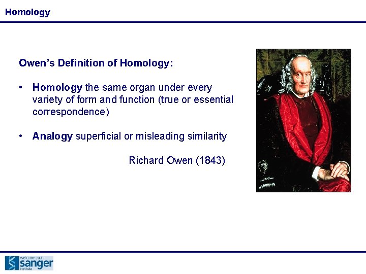
Homology Owen’s Definition of Homology: • Homology the same organ under every variety of form and function (true or essential correspondence) • Analogy superficial or misleading similarity Richard Owen (1843)

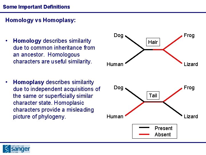
Some Important Definitions Homology vs Homoplasy: • Homology describes similarity due to common inheritance from an ancestor. Homologous characters are useful similarity. • Homoplasy describes similarity due to independent acquisitions of the same or superficially similar character state. Homoplasic characters provide a misleading picture of phylogeny. Dog Frog Hair Human Lizard Dog Frog Tail Human Lizard Present Absent

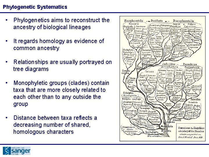
Phylogenetic Systematics • Phylogenetics aims to reconstruct the ancestry of biological lineages • It regards homology as evidence of common ancestry • Relationships are usually portrayed on tree diagrams • Monophyletic groups (clades) contain taxa that are more closely related to each other than to any outside the group • Distance between taxa reflects a decreasing number of shared, homologous characters

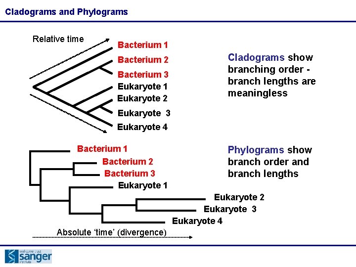
Cladograms and Phylograms Relative time Bacterium 1 Bacterium 2 Bacterium 3 Eukaryote 1 Eukaryote 2 Cladograms show branching order branch lengths are meaningless Eukaryote 3 Eukaryote 4 Bacterium 1 Bacterium 2 Bacterium 3 Eukaryote 1 Phylograms show branch order and branch lengths Eukaryote 2 Eukaryote 3 Eukaryote 4 Absolute ‘time’ (divergence)

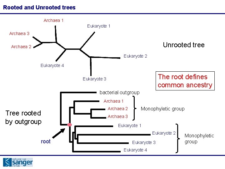
Rooted and Unrooted trees Archaea 1 Eukaryote 1 Archaea 3 Unrooted tree Archaea 2 Eukaryote 4 The root defines common ancestry Eukaryote 3 bacterial outgroup Archaea 1 Tree rooted by outgroup Archaea 2 Monophyletic group Archaea 3 Eukaryote 1 Eukaryote 2 root Eukaryote 3 Eukaryote 4 Monophyletic group

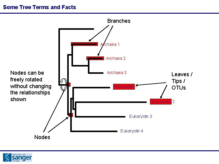
Some Tree Terms and Facts Branches Archaea 1 Archaea 2 Nodes can be freely rotated without changing the relationships shown Archaea 3 Leaves / Tips / OTUs Eukaryote 1 Eukaryote 2 Eukaryote 3 Eukaryote 4 Nodes

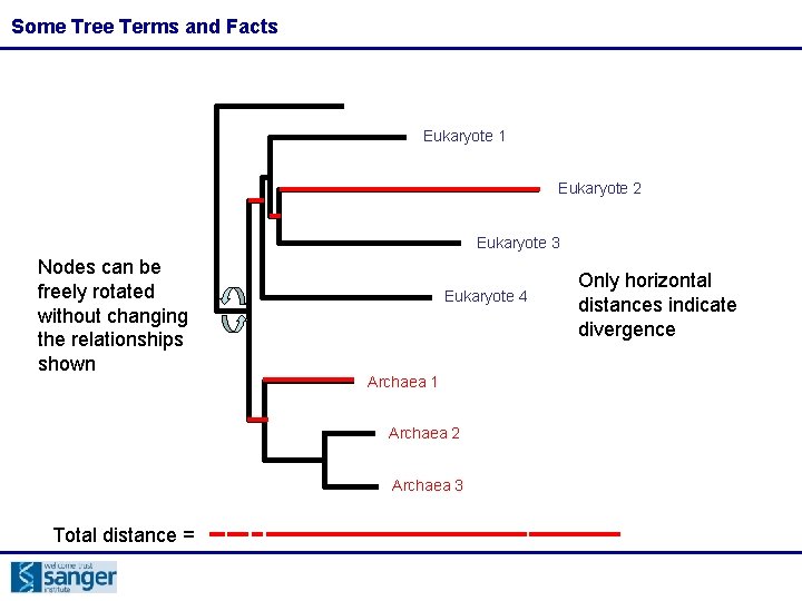
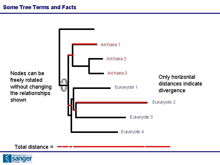
Some Tree Terms and Facts Eukaryote 1 Eukaryote 2 Eukaryote 3 Nodes can be freely rotated without changing the relationships shown Eukaryote 4 Archaea 1 Archaea 2 Archaea 3 Total distance = Only horizontal distances indicate divergence

Some Tree Terms and Facts Archaea 1 Archaea 2 Nodes can be freely rotated without changing the relationships shown Archaea 3 Only horizontal distances indicate divergence Eukaryote 1 Eukaryote 2 Eukaryote 3 Eukaryote 4 Total distance =

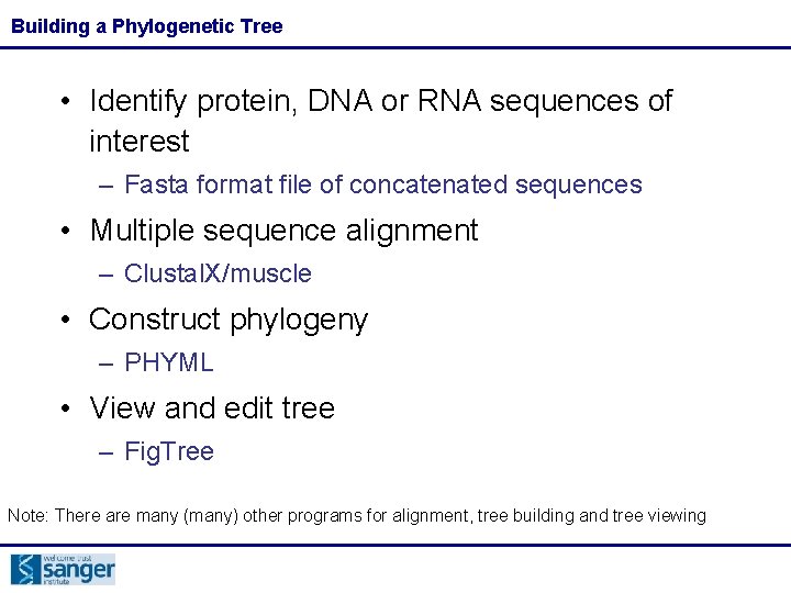
Building a Phylogenetic Tree • Identify protein, DNA or RNA sequences of interest – Fasta format file of concatenated sequences • Multiple sequence alignment – Clustal. X/muscle • Construct phylogeny – PHYML • View and edit tree – Fig. Tree Note: There are many (many) other programs for alignment, tree building and tree viewing

Multiple Alignments • An alignment is a hypothesis of positional homology between bases/amino acids of different sequences • Phylogeny is meaningless unless it is based on a well-made alignment

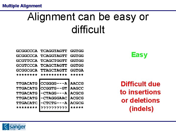
Multiple Alignment can be easy or difficult Easy Difficult due to insertions or deletions (indels)

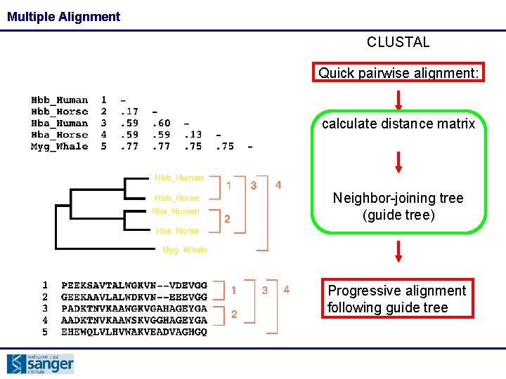
Multiple Alignment CLUSTAL Quick pairwise alignment: calculate distance matrix Neighbor-joining tree (guide tree) Progressive alignment following guide tree

Building a Phylogenetic Tree Choices are Unavoidable! • There are many different phylogenetic methods • So, you will be confronted with unavoidable choices • Not all methods are equally good for all data • Although we do not need to understand all the details of the various phylogenetic methods, an understanding of the basic properties is essential for informed choice of method and interpretation of results

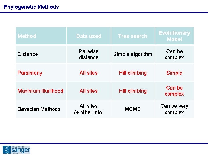
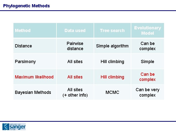
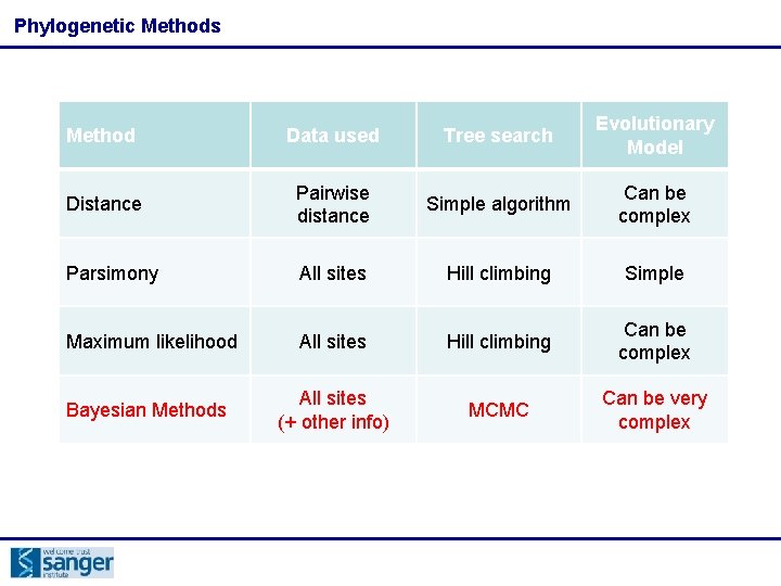
Phylogenetic Methods Method Data used Tree search Evolutionary Model Distance Pairwise distance Simple algorithm Can be complex Parsimony All sites Hill climbing Simple Maximum likelihood All sites Hill climbing Can be complex Bayesian Methods All sites (+ other info) MCMC Can be very complex

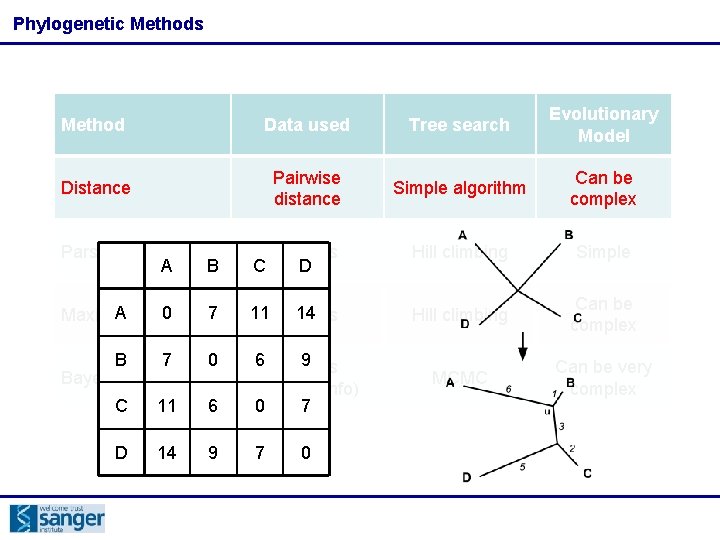
Phylogenetic Methods Method Data used Tree search Evolutionary Model Distance Pairwise distance Simple algorithm Can be complex B All sites C D Hill climbing Simple A likelihood 0 7 Maximum 11 All 14 sites Hill climbing Can be complex B 7 0 Bayesian Methods MCMC Can be very complex Parsimony A C 11 6 6 All 9 sites (+ other info) 0 7 D 14 9 7 0

Phylogenetic Methods Method Data used Tree search Evolutionary Model Distance Pairwise distance Simple algorithm Can be complex Parsimony All sites Hill climbing Simple Maximum likelihood All sites Hill climbing Can be complex Bayesian Methods All sites (+ other info) MCMC Can be very complex

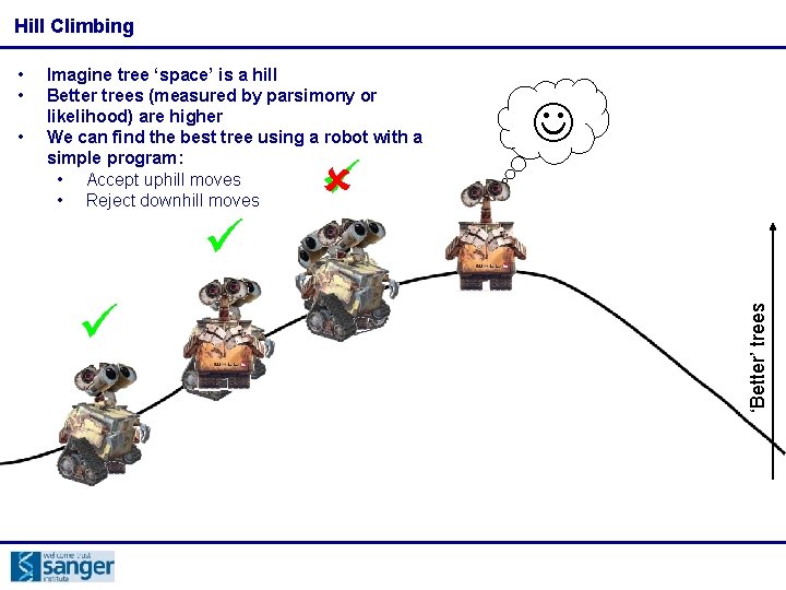
Hill Climbing • Imagine tree ‘space’ is a hill Better trees (measured by parsimony or likelihood) are higher We can find the best tree using a robot with a simple program: • Accept uphill moves • Reject downhill moves ‘Better’ trees • •

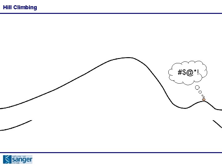
Hill Climbing #$@*!

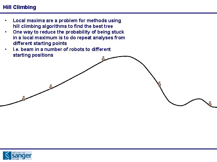
Hill Climbing • • • Local maxima are a problem for methods using hill climbing algorithms to find the best tree One way to reduce the probability of being stuck in a local maximum is to do repeat analyses from different starting points I. e. beam in a number of robots to different starting positions

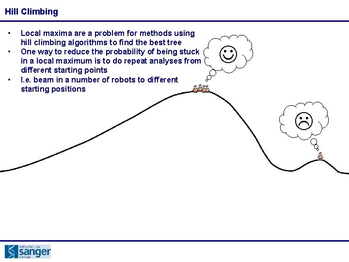
Hill Climbing • • • Local maxima are a problem for methods using hill climbing algorithms to find the best tree One way to reduce the probability of being stuck in a local maximum is to do repeat analyses from different starting points I. e. beam in a number of robots to different starting positions

Phylogenetic Methods Method Data used Tree search Evolutionary Model Distance Pairwise distance Simple algorithm Can be complex Parsimony All sites Hill climbing Simple Maximum likelihood All sites Hill climbing Can be complex Bayesian Methods All sites (+ other info) MCMC Can be very complex

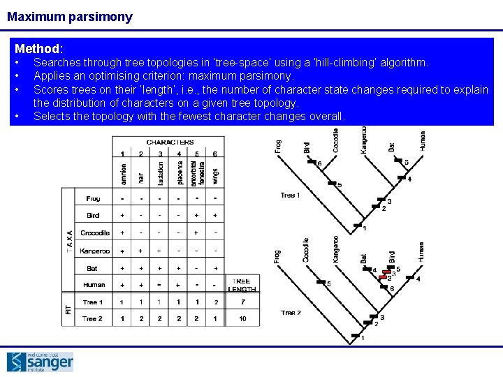
Maximum parsimony Method: • • Searches through tree topologies in ‘tree-space’ using a ‘hill-climbing’ algorithm. Applies an optimising criterion: maximum parsimony. Scores trees on their ‘length’, i. e. , the number of character state changes required to explain the distribution of characters on a given tree topology. Selects the topology with the fewest character changes overall.

Phylogenetic Methods Method Data used Tree search Evolutionary Model Distance Pairwise distance Simple algorithm Can be complex Parsimony All sites Hill climbing Simple Maximum likelihood All sites Hill climbing Can be complex Bayesian Methods All sites (+ other info) MCMC Can be very complex

Likelihood The Idiot’s Guide to the Zen of Likelihood in a Nutshell in Seven Days for Dummies, Unleashed A gentle introduction, for those of us who are small of brain, to the calculation of the likelihood of molecular sequences. http: //www. bmnh. org/web_users/pf/idiots. pdf

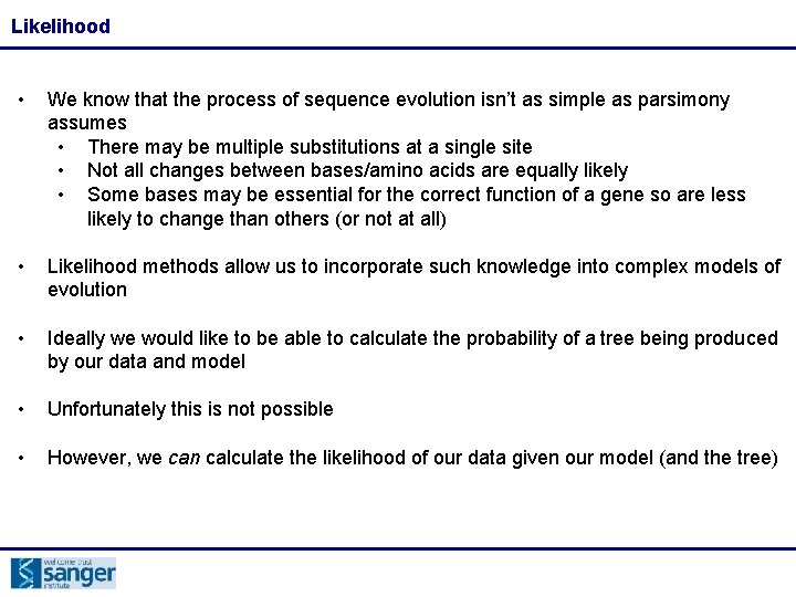
Likelihood • We know that the process of sequence evolution isn’t as simple as parsimony assumes • There may be multiple substitutions at a single site • Not all changes between bases/amino acids are equally likely • Some bases may be essential for the correct function of a gene so are less likely to change than others (or not at all) • Likelihood methods allow us to incorporate such knowledge into complex models of evolution • Ideally we would like to be able to calculate the probability of a tree being produced by our data and model • Unfortunately this is not possible • However, we can calculate the likelihood of our data given our model (and the tree)

Likelihood • Imagine tossing a coin and getting a head. What is the probability (likelihood) of that result?

Likelihood • Imagine tossing a coin and getting a head. What is the probability (likelihood) of that result? • If our model is that the coin is fair, the probability is 0. 5 • If our model is a double headed coin, the probability is 1 • The model you choose can have a big effect on the likelihood

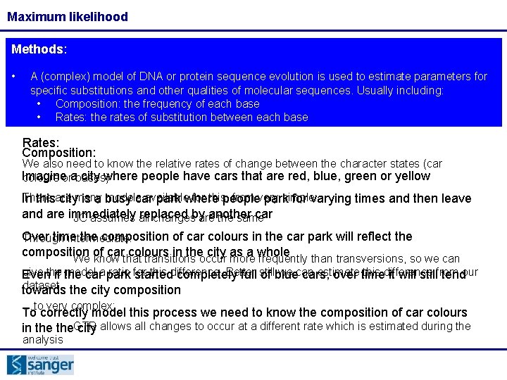
Maximum likelihood Methods: • A (complex) model of DNA or protein sequence evolution is used to estimate parameters for specific substitutions and other qualities of molecular sequences. Usually including: • Composition: the frequency of each base • Rates: the rates of substitution between each base Rates: Composition: We also need to know the relative rates of change between the character states (car Imagine city where people have cars that are red, blue, green or yellow colours orabases) There models available for this, from very simple: In thisare citymany is a busy car park where people park for varying times and then leave and are immediately replaced another car JC assumes all changesby are the same Over time the composition of car colours in the car park will reflect the Through intermediate: composition of car colours in the city as a whole We know that transitions occur more frequently than transversions, so we can give the model ratio for this difference. Better we can estimate this difference Even if the cara park started completely full still of blue cars, over time it will stillfrom tendour dataset the city composition towards …to very complex: To correctly model this process we need to know the composition of car colours in the. GTR city allows all changes to occur at a different rate which is estimated during the analysis

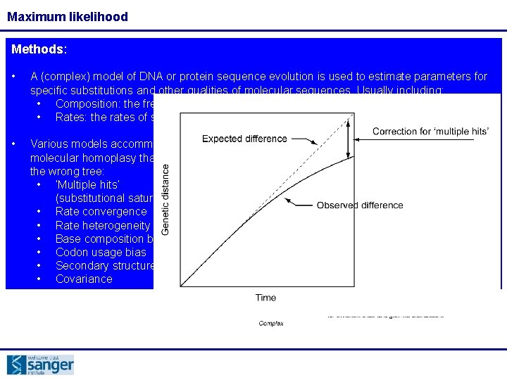
Maximum likelihood Methods: • A (complex) model of DNA or protein sequence evolution is used to estimate parameters for specific substitutions and other qualities of molecular sequences. Usually including: • Composition: the frequency of each base • Rates: the rates of substitution between each base • Various models accommodate sources of molecular homoplasy that might result in the wrong tree: • ‘Multiple hits’ (substitutional saturation) • Rate convergence • Rate heterogeneity • Base composition bias • Codon usage bias • Secondary structure • Covariance

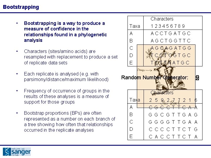
Bootstrapping • • Bootstrapping is a way to produce a measure of confidence in the relationships found in a phylogenetic analysis Characters (sites/amino acids) are resampled with replacement to produce a set of replicate data sets • Each replicate is analysed (e. g. with parsimony/distance/maximum likelihood) • Frequency of occurrence of groups in the results of these analyses is a measure of support for those groups • Bootstrap proportions (BPs) are often represented as a number on each branch of a tree showing how often that relationships occurred in the replicate analyses Characters Taxa 123456789 A ACCTGATGC B AGCTGGTTC C AGCAGATGG D TCCTCGTGC E TCTTAATGC Random Number Generator: 9 5 2 Characters Taxa 2 5 9 2 7 7 2 1 6 A C G C C T T C A A B G G C G T T G A G C G G T T G A A D C C T T C T G E C A C C T T C T A

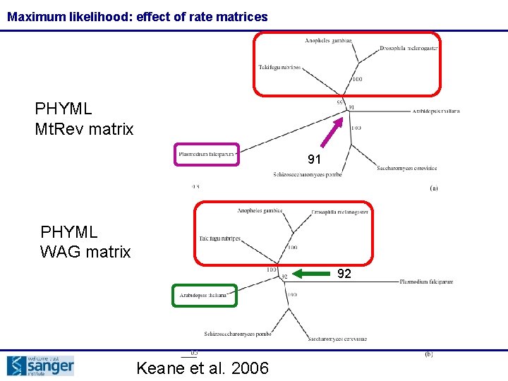
Maximum likelihood: effect of rate matrices PHYML Mt. Rev matrix 91 PHYML WAG matrix 92 Keane et al. 2006

Phylogenetic Methods Method Data used Tree search Evolutionary Model Distance Pairwise distance Simple algorithm Can be complex Parsimony All sites Hill climbing Simple Maximum likelihood All sites Hill climbing Can be complex Bayesian Methods All sites (+ other info) MCMC Can be very complex

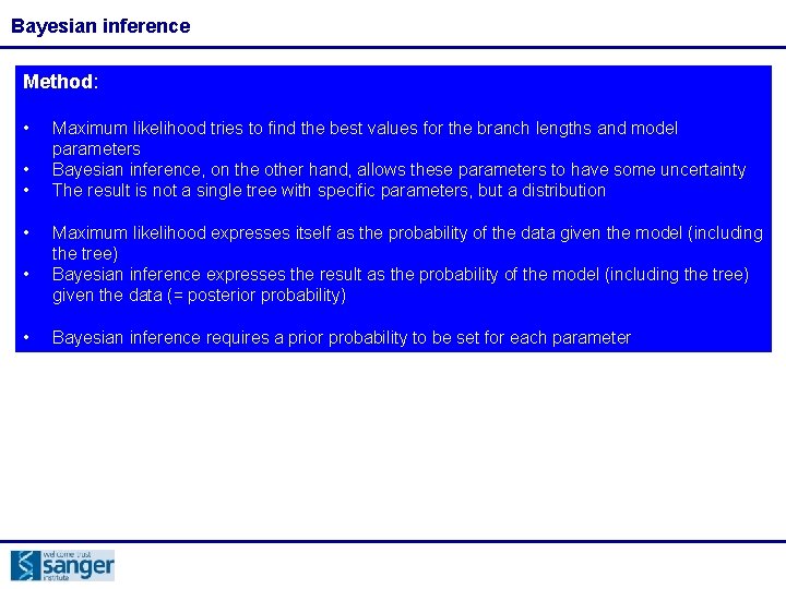
Bayesian inference Method: • • • Maximum likelihood tries to find the best values for the branch lengths and model parameters Bayesian inference, on the other hand, allows these parameters to have some uncertainty The result is not a single tree with specific parameters, but a distribution Maximum likelihood expresses itself as the probability of the data given the model (including the tree) Bayesian inference expresses the result as the probability of the model (including the tree) given the data (= posterior probability) Bayesian inference requires a prior probability to be set for each parameter

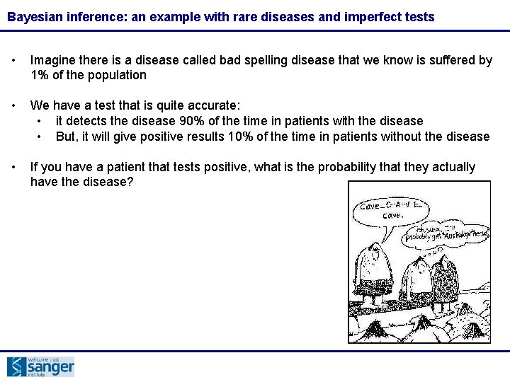
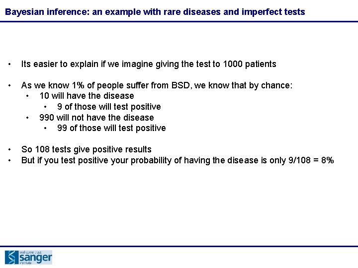
Bayesian inference: an example with rare diseases and imperfect tests • Imagine there is a disease called bad spelling disease that we know is suffered by 1% of the population • We have a test that is quite accurate: • it detects the disease 90% of the time in patients with the disease • But, it will give positive results 10% of the time in patients without the disease • If you have a patient that tests positive, what is the probability that they actually have the disease?

Bayesian inference: an example with rare diseases and imperfect tests • Its easier to explain if we imagine giving the test to 1000 patients • As we know 1% of people suffer from BSD, we know that by chance: • 10 will have the disease • 9 of those will test positive • 990 will not have the disease • 99 of those will test positive • • So 108 tests give positive results But if you test positive your probability of having the disease is only 9/108 = 8%

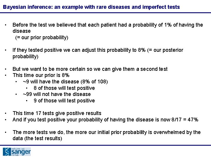
Bayesian inference: an example with rare diseases and imperfect tests • Before the test we believed that each patient had a probability of 1% of having the disease (= our prior probability) • If they tested positive we can adjust this probability to 8% (= our posterior probability) • • But we want to be more certain so we can give them a second test This time our prior is 8% • ~9 will have the disease (8% of 108) • 8 of those will test positive • ~99 will not have the disease • 9 of those will test positive • • This time 17 tests give positive results And if you test positive your probability of having the disease is now 8/17 = 47% • The more tests we do, the more our initial prior probability is overwhelmed by the data (the test results)

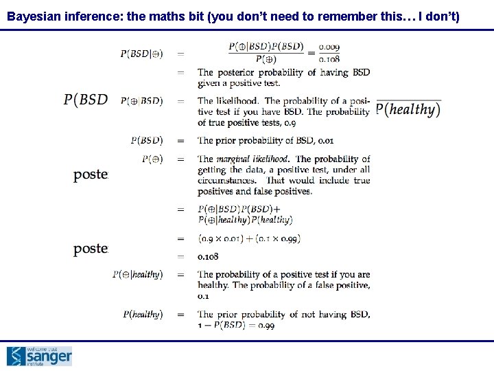
Bayesian inference: the maths bit (you don’t need to remember this… I don’t)

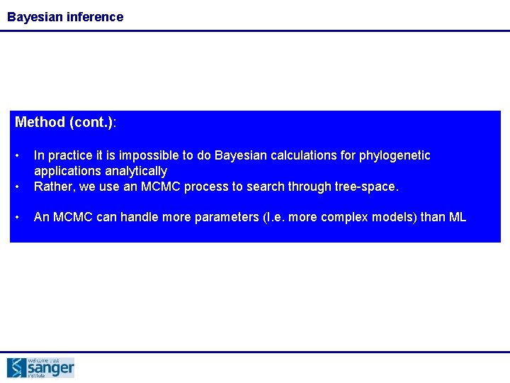
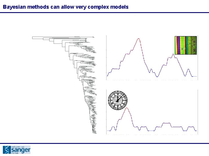
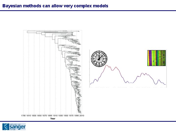
Bayesian inference Method (cont. ): • • In practice it is impossible to do Bayesian calculations for phylogenetic applications analytically Rather, we use an MCMC process to search through tree-space. • An MCMC can handle more parameters (I. e. more complex models) than ML

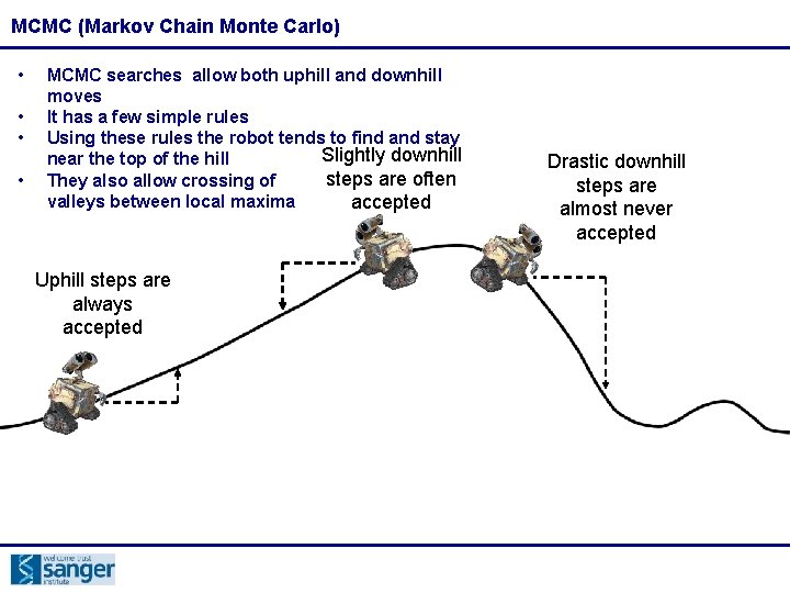
MCMC (Markov Chain Monte Carlo) • • MCMC searches allow both uphill and downhill moves It has a few simple rules Using these rules the robot tends to find and stay Slightly downhill near the top of the hill steps are often They also allow crossing of valleys between local maxima accepted Uphill steps are always accepted Drastic downhill steps are almost never accepted

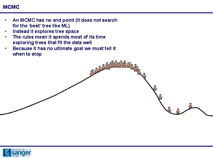
MCMC • • An MCMC has no end point (it does not search for the ‘best’ tree like ML) Instead it explores tree space The rules mean it spends most of its time exploring trees that fit the data well Because it has no ultimate goal we must tell it when to stop

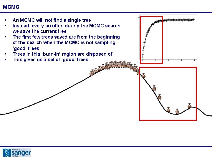
MCMC • • • An MCMC will not find a single tree Instead, every so often during the MCMC search we save the current tree The first few trees saved are from the beginning of the search when the MCMC is not sampling ‘good’ trees Trees in this ‘burn-in’ region are disposed of This gives us a set of ‘good’ trees

Bayesian methods can allow very complex models

Bayesian methods can allow very complex models

Bayesian methods can allow very complex models

Further details Textbooks: Hall Phylogenetic trees made easy. Sinauer Associates. Page & Holmes Molecular Evolution: A Phylogenetic Approach. Blackwell Science. Felsenstein Inferring Phylogenies. Sinauer Associates. Software: Phyml http: //atgc. lirmm. fr/phyml/ PAUP* (NJ, MP, ML): http: //paup. csit. fdsu. edu PHYLIP (NJ, MP, ML): http: //evolution. genetics. washington. edu/phylip. html Mr. Bayes (Bayesian): http: //mrbayes. csit. fdsu. edu Splitstree (Networks): http: //www. splitstree. org Find. Model (Model Test): http: //www. hiv. lanl. gov/content/sequence/findmodel. html Sea. View (Contains Clustal, Muscle, PHYLIP and Phy. ML + a simple tree viewer: http: //pbil. univ-lyon 1. fr/software/seaview. html Websites: Multi. Phyl (ML via email): http: //distributed. cs. nuim. ie/multiphyl. php Phylogeny. fr (Robust Phylogenetic Analysis For The Non-Specialist): http: //www. phylogeny. fr/ Felsenstein’s Phylogeny program page (links to available software): http: //evolution. genetics. washington. edu/phylip/software. html