WellBalanced FiniteVolume Model for LongWave Runup NCTR Seminar

Well-Balanced Finite-Volume Model for Long-Wave Runup NCTR Seminar Yong Wei May 21, 2007

Tsunami in the Coasts Flow Velocity Flow Depth § § Inundation and runup Water level (Flow depth) Flow velocity (Current speed) A good runup model should describe all these quantities within a 15% error margin (Shuto, 1991) with accurate local bathymetry and topography

Challenges of Long-Wave Runup Models § Volume conservation “Conservative numerical methods, if convergent, do converge to correct solution of the equations” - Lax and Wendoff (1960) § Discontinuous flow “If a non-conservative method is used, then the wrong solution will be computed, if it contains a shock wave” - Hou and Le. Floch (1994) § Moving wet/dry boundary

Finite-Volume Model of Godunov Type § § § Conservative numerical scheme Based on integral, conservative NLSW Godunov-type method: Riemann solutions Explicit upwind scheme Well known to deal with volume conservation and flow discontinuity § Riemann problem provides solutions for moving boundary

Finite-Volume Formulation § Conservative form of NLSW § Integrate over a control volume

Time Integration § Flux terms F and G are obtained using Riemann solution § Direct solutions are not available for two or higherdimensional exact Riemann problems § Present model uses a second-order splitting scheme for time integration

Well-Balanced Scheme and Surface Gradient Method (SGM) h i-1/2 H SGM i i+1/2 DGM i+1 § Well-balance scheme: keeps U = 0, = const exactly for still flow § Surface Gradient Method (Zhou et al. , 2001) § SGM defines bathy and topo at the cell interface § SGM reconstructs cell-interface flow depth by piecewise linear interpolating , i± 1/2 = i ± 1/2∆x i § SGM is a well-balanced scheme and eliminates inaccuracies due to bed slope

Slope Limiter § Spurious oscillations in the vicinity of high gradients are expected § Slope limiter is used to limit the spatial derivatives to realistic values

Exact Riemann Problem Interface § Generalization of dam -break problem § The solution of 1 D exact Riemann problem is known t= t* Star Region Shock Rarefaction x=0

Moving Waterline § Wet/dry Riemann problem § Minimum wet depth approach is more robust and efficient

Model Verification and Validation § Verification using analytical solutions v Frictionless tidal flow v Periodic wave reflection from a plane beach v Long-wave resonance in a circular parabolic basin § Validation using laboratory measurements v Solitary wave runup on a plane beach v Solitary wave runup on a circular island v Tsunami runup onto a complex 3 D beach: Catalina Tsunami Workshop Benchmark 2

Well-Balanced Scheme § A frictionless tidal flow over varying bathymetry (Bermudez and Vazquez, 1994)

Periodic Wave Reflection from a Plane Beach § Carrier and Greenspan (1958)

Long-Wave Resonance in a Circular Parabolic Basin § Thacker (1981)

Solitary Wave Runup on Plane Beach § Series of experiments v Various steep slope (Hall and Watts, 1953) v 1: 19. 85 (Synolakis, 1987) v 1: 15 (Li and Raichlen, 2002) § Asymptotic Solutions v R/h = 2. 831(cos )1/2(A/h)5/4 (Synolakis, 1987) v R/h = 2. 831(cos )1/2(A/h)5/4+ 0. 293(cos )3/2(A/h)9/4 (Li and Raichlen, 2002)

, Synolakis’ experiments (1987); · · ·, Zelt (1991); -- - -, Titov and Synolakis (1995); , Li and Raichlen (2002); , present finite-volume model

Volume Conservation Error = (V-V 0)/V 0 t/(g/h)1/2

Solitary Wave Runup on Different Slopes , Hall and Watts (1953); 1: 5. 67 1: 19. 85 1: 15 , Synolakis (1987); , Li and Raichlen (2002). Shallow-water models: , Li and Raichlen (2002); - - -, Li and Raichlen (2001); , present finite volume model.

Solitary Wave on a Conical Island (Briggs et al. , 1995)

Time Series Comparison Left: A/h = 0. 1 Right: A/h = 0. 2 , Briggs et al. (1995); , present model;

Inundation Limits around the Island A/h = 0. 1 A/h = 0. 2

Tsunami Runup onto a Complex 3 D Beach § Numerical Domain: § § 5. 448 m X 3. 402 m Minimum depth: -0. 125 m (land) Maximum depth: 0. 13535 m Grid size 0. 014 m § Boundary conditions: § § § West: input wave North: solid wall East: solid wall § South: solid wall § Input wave:

Comparison of inundation

Modeling Tsunami Waves § Case study: 1946 Alaska-Aleutian tsunami § COMCOT (Liu et al. 1995) computes tsunami propagation in the open ocean § The present finite-volume model computes the runup and inundation at specific site

Topography & Bathymetry Sources Resolution Coverage Agencies GEBCO 1 min Global British Oceanographic Data Center ETOPO 2 2 min Global NGDC GEBCO-ETOPO 2 mixing 1 min Global NOAA Coastal Relief (US) 3 sec US NGDC Hawaiian Regional Bathymetry 5 sec Hawaii JAMSTEC and USGS SHOALS 4 m Shore to -40 m USACE DEM 10 ~ 30 m Global USGS Photogrammetric Data 5 ft (vertical) Oahu & Hilo City & County Li. DAR Topography 2 m US NOAA CSC GPS data 2 m Parts of Oahu ORE

Surface Roughness § Bretschneider et al. (1986) provides Manning’s number for a variety of terrains along Hawaiian coasts. § Friction grids are developed using aerial photos and Arc. GIS Mokuleia Friction Grid

COMCOT Computation

Haleiwa: Bathymetry and Topography

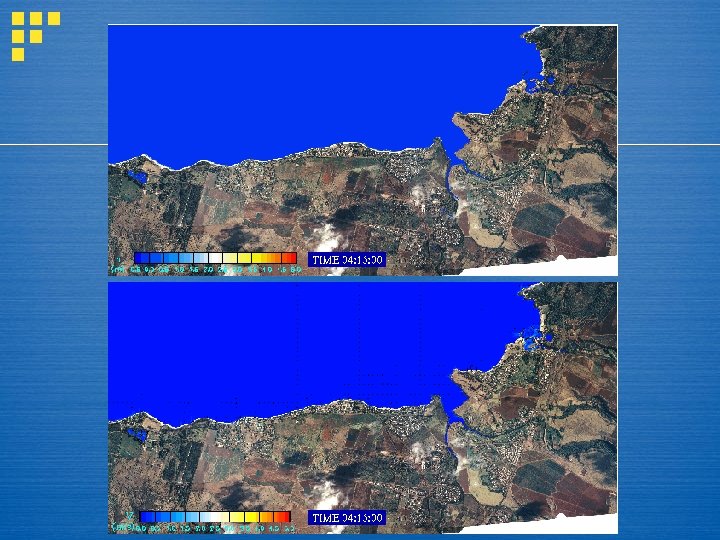
Computed Runup and Inundation at Haleiwa ● = locations of observed runup; █ = observed runup; ● = computed runup; dark blue shade = computed inundation.

Mokuleia

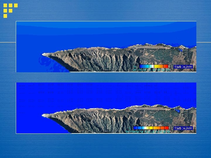
Computed Runup and Inundation at Mokuleia Courtesy of Dan Walker. ● = locations of observed runup; █ = observed runup; ● = computed runup; dark blue shade = computed inundation.

Conclusions Satisfies the well-balance criteria n Excellent volume conservation ability n Demonstrates good shock-capturing capability n Provides good approximation of a breaking wave as a propagating bore n Shows very good agreement with analytical solutions and laboratory measurements n

Future Work § Modeling tsunami propagation and inundation: nested or curvilinear? § Comparative study with MOST: more benchmarks? § Upgrade to Boussinesq-type model for more applications: tsunami waves, storm waves, ship waves … § Includes more module: Asteroid impact, landslide, sediment transport …