Welcome to Daves Data Demonstration This presentation is

Welcome to Dave’s Data Demonstration • This presentation is designed for users of SPSS with some familiarity with the program and a willingness to experiment with the syntax editor. If you’re new to the software, take a deep breath and relax, there are screenshots to guide you and items that you can simply cut and paste if you need to.

A few things to start • A few basic commands to know: – The paste button on the interface opens up the syntax editor and pastes what you’ve done onto that. This is your friend when you’re creating data. – In order for SPSS to know how big a set you want, create your variables in variable view first, then using data view, input a dummy value in the row representing your last participant. This sets the sample size for you very easily. – Keep variable names simple and short, it will save you quite a bit of time.

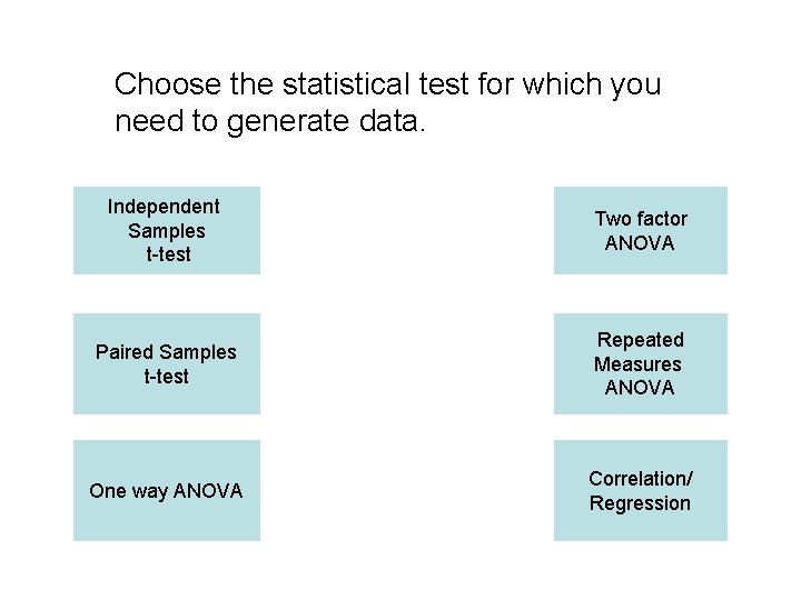
Choose the statistical test for which you need to generate data. Independent Samples t-test Two factor ANOVA Paired Samples t-test Repeated Measures ANOVA One way ANOVA Correlation/ Regression

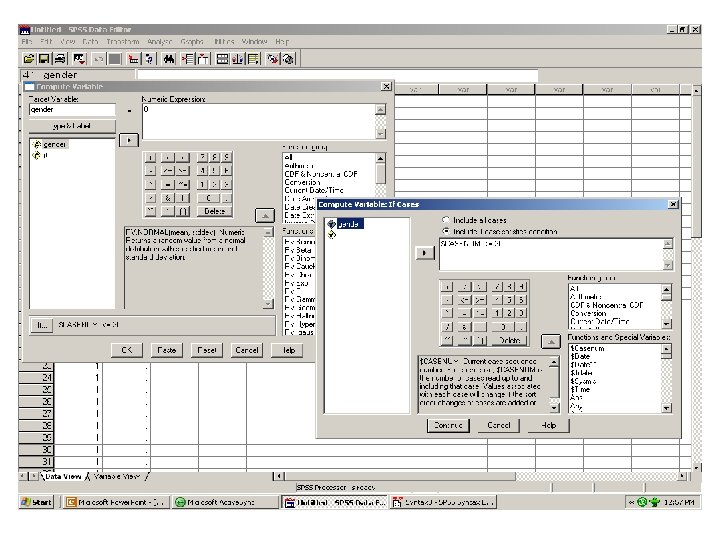
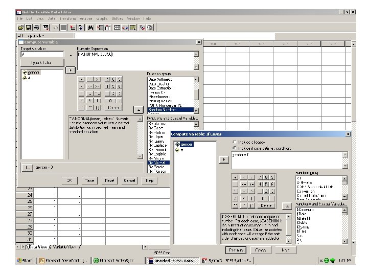
Independent samples t-test • What you need… • Column one: Grouping variable • Column two: Dependent variable The next slides show you what the SPSS window will look like using the Transform Compute command followed by selecting the “If” button. First is the sequence of commands to generate the grouping variable, second is the commands for the dependent variable.

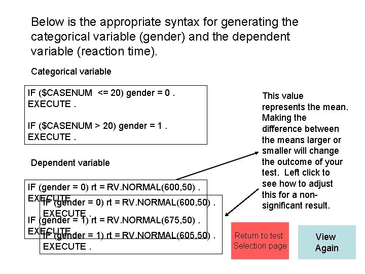
Below is the appropriate syntax for generating the categorical variable (gender) and the dependent variable (reaction time). Categorical variable IF ($CASENUM <= 20) gender = 0. EXECUTE. IF ($CASENUM > 20) gender = 1. EXECUTE. Dependent variable IF (gender = 0) rt = RV. NORMAL(600, 50). EXECUTE. = 0) rt = RV. NORMAL(600, 50). IF (gender EXECUTE. IF (gender = 1) rt = RV. NORMAL(675, 50). EXECUTE. = 1) rt = RV. NORMAL(605, 50). IF (gender EXECUTE. This value represents the mean. Making the difference between the means larger or smaller will change the outcome of your test. Left click to see how to adjust this for a nonsignificant result. Return to test Selection page View Again

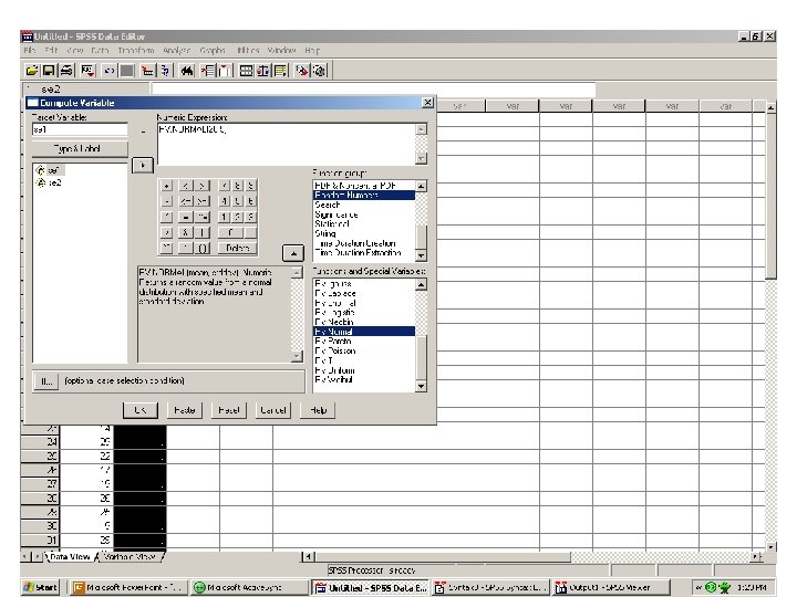
Paired samples t-test • What you need – One dependent variable (DV) measured twice for the same participants – Column one: DV time one – Column two: DV time two The next slide shows you what the SPSS window will look like using the Transform Compute command. Repeat the exact same process for both variables.

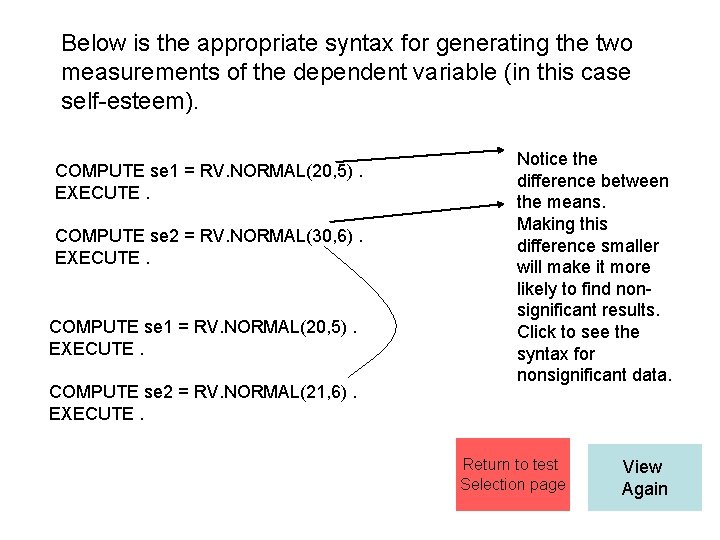
Below is the appropriate syntax for generating the two measurements of the dependent variable (in this case self-esteem). COMPUTE se 1 = RV. NORMAL(20, 5). EXECUTE. COMPUTE se 2 = RV. NORMAL(30, 6). EXECUTE. COMPUTE se 1 = RV. NORMAL(20, 5). EXECUTE. COMPUTE se 2 = RV. NORMAL(21, 6). EXECUTE. Notice the difference between the means. Making this difference smaller will make it more likely to find nonsignificant results. Click to see the syntax for nonsignificant data. Return to test Selection page View Again

One way ANOVA • Data creation for a one way ANOVA is an identical process to the Independent Samples ttest. Click on the button below to view the screenshots for the independent samples case if you’d like to review it. • The next slide contains the syntax information for a significant one way ANOVA. Independent Samples T-test Syntax for One-way ANOVA

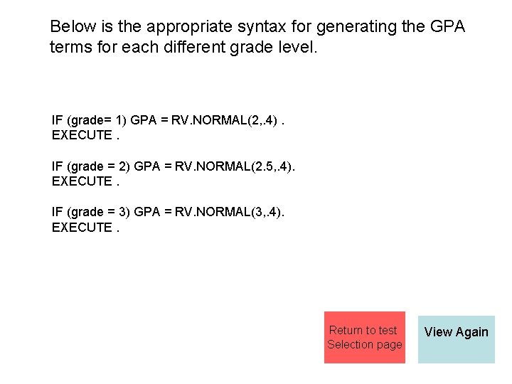
Below is the appropriate syntax for generating the GPA terms for each different grade level. IF (grade= 1) GPA = RV. NORMAL(2, . 4). EXECUTE. IF (grade = 2) GPA = RV. NORMAL(2. 5, . 4). EXECUTE. IF (grade = 3) GPA = RV. NORMAL(3, . 4). EXECUTE. Return to test Selection page View Again

Two factor ANOVA • Generating good Two factor ANOVA data can be tricky. However, the main thing to remember is that you want to create your data in a cell by cell fashion. With a little good old fashion pencil and paper planning, you can lay out main effects and interactions and then use “If” commands to fill things in cell by cell.

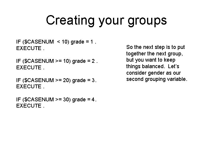
Creating your groups IF ($CASENUM < 10) grade = 1. EXECUTE. IF ($CASENUM >= 10) grade = 2. EXECUTE. IF ($CASENUM >= 20) grade = 3. EXECUTE. IF ($CASENUM >= 30) grade = 4. EXECUTE. So the next step is to put together the next group, but you want to keep things balanced. Let’s consider gender as our second grouping variable.

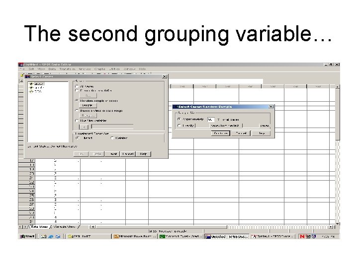
The second grouping variable…

The second grouping variable By selecting approximately 50% of the cases, this creates a new filter variable. Then, it is simple cutting and pasting to move the numbers from the filter column into the gender column. After you cut and paste, then turn select cases off and you’ve got gender distributed across the whole set.

Finally, it’s just a matter of writing the syntax for your random normally distributed dependent variable IF (grade = 1 and gender = 0) GPA = RV. NORMAL (2, . 4). EXECUTE. IF (grade = 1 and gender = 1) GPA = RV. NORMAL (2. 4, . 4). EXECUTE. IF (grade = 2 and gender = 0) GPA = RV. NORMAL (2. 4, . 4). EXECUTE. IF (grade = 2 and gender = 1) GPA = RV. NORMAL (2. 6, . 4). EXECUTE. IF (grade = 3 and gender = 0) GPA = RV. NORMAL (3, . 4). EXECUTE. IF (grade = 3 and gender = 1) GPA = RV. NORMAL (2. 9, . 4). EXECUTE. IF (grade = 4 and gender = 0) GPA = RV. NORMAL (3. 1, . 4). EXECUTE. IF (grade = 4 and gender = 1) GPA = RV. NORMAL (3. 2, . 4). EXECUTE. Return to test Selection page View Again

Repeated Measures ANOVA • Data creation for a repeated measures ANOVA is an identical process to the Paired Samples ttest. Click on the button below to view the screenshots for the paired samples case if you’d like to review it. • The next slide contains the syntax information for a significant one way ANOVA. Paired Samples T-test Syntax for repeated measures ANOVA

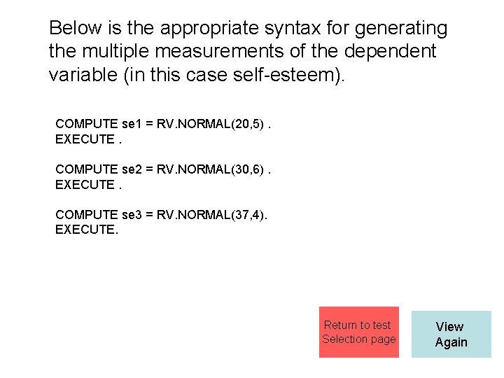
Below is the appropriate syntax for generating the multiple measurements of the dependent variable (in this case self-esteem). COMPUTE se 1 = RV. NORMAL(20, 5). EXECUTE. COMPUTE se 2 = RV. NORMAL(30, 6). EXECUTE. COMPUTE se 3 = RV. NORMAL(37, 4). EXECUTE. Return to test Selection page View Again

Correlation/Regression • Correlational data is slightly different to create. In most other situations, we’re comparing means with each other. In the case of correlation, we have to construct the dataset in such a way as to reflect the relationship in the data. No longer can we just change mean values of normal distributions. • The next slides contain the screenshots for the creation of the correlational data as well as the syntax for a pairwise comparison.

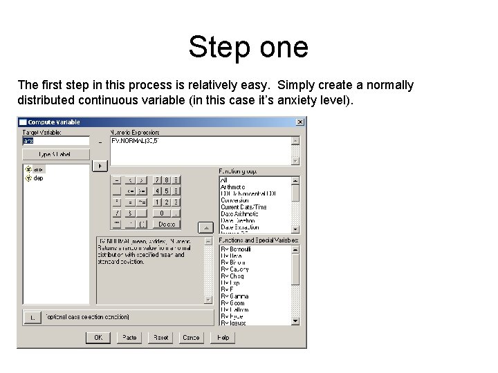
Step one The first step in this process is relatively easy. Simply create a normally distributed continuous variable (in this case it’s anxiety level).

Step two • In this step you have to establish the relationship between the variables. The key is to create the next variable (depression) in such a way that anxiety plays a role in its creation.

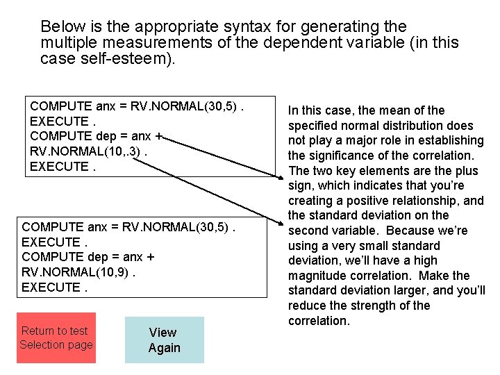
Below is the appropriate syntax for generating the multiple measurements of the dependent variable (in this case self-esteem). COMPUTE anx = RV. NORMAL(30, 5). EXECUTE. COMPUTE dep = anx + RV. NORMAL(10, . 3). EXECUTE. COMPUTE anx = RV. NORMAL(30, 5). EXECUTE. COMPUTE dep = anx + RV. NORMAL(10, 9). EXECUTE. Return to test Selection page View Again In this case, the mean of the specified normal distribution does not play a major role in establishing the significance of the correlation. The two key elements are the plus sign, which indicates that you’re creating a positive relationship, and the standard deviation on the second variable. Because we’re using a very small standard deviation, we’ll have a high magnitude correlation. Make the standard deviation larger, and you’ll reduce the strength of the correlation.