Weighted k NN clustering trees and Bayesian classification

Weighted k. NN, ~ clustering, trees and Bayesian classification Peter Fox Data Analytics – ITWS-4963/ITWS-6965 Week 5 a, February 24, 2015 1

Plot tools/ tips http: //statmethods. net/advgraphs/layout. html http: //flowingdata. com/2014/02/27/how-to-read-histograms-and-use-them-inr/ pairs, gpairs, scatterplot. matrix, clustergram, etc. data() # precip, presidents, iris, swiss, sunspot. month (!), environmental, ethanol, ionosphere More script fragments in R will be available on the web site (http: //escience. rpi. edu/data/DA ) 2

Weighted KNN? require(kknn) data(iris) m <- dim(iris)[1] val <- sample(1: m, size = round(m/3), replace = FALSE, prob = rep(1/m, m)) iris. learn <- iris[-val, ] iris. valid <- iris[val, ] iris. kknn <- kknn(Species~. , iris. learn, iris. valid, distance = 1, kernel = "triangular") summary(iris. kknn) fit <- fitted(iris. kknn) table(iris. valid$Species, fit) pcol <- as. character(as. numeric(iris. valid$Species)) pairs(iris. valid[1: 4], pch = pcol, col = c("green 3", "red”)[(iris. valid$Species != fit)+1]) 3

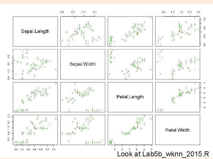
4 Look at Lab 5 b_wknn_2015. R

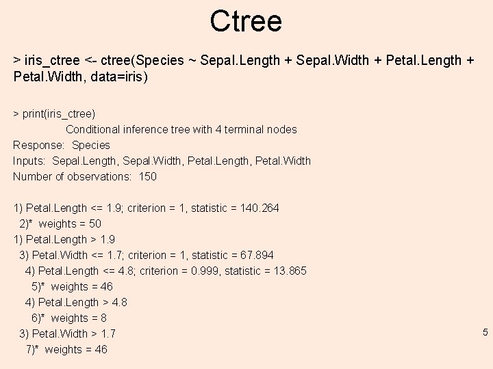
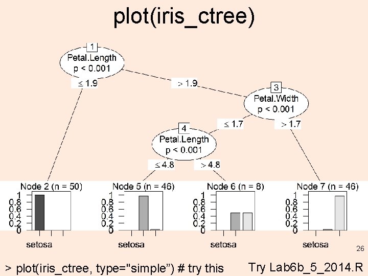
Ctree > iris_ctree <- ctree(Species ~ Sepal. Length + Sepal. Width + Petal. Length + Petal. Width, data=iris) > print(iris_ctree) Conditional inference tree with 4 terminal nodes Response: Species Inputs: Sepal. Length, Sepal. Width, Petal. Length, Petal. Width Number of observations: 150 1) Petal. Length <= 1. 9; criterion = 1, statistic = 140. 264 2)* weights = 50 1) Petal. Length > 1. 9 3) Petal. Width <= 1. 7; criterion = 1, statistic = 67. 894 4) Petal. Length <= 4. 8; criterion = 0. 999, statistic = 13. 865 5)* weights = 46 4) Petal. Length > 4. 8 6)* weights = 8 3) Petal. Width > 1. 7 7)* weights = 46 5

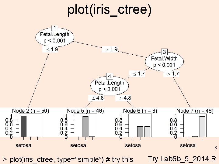
plot(iris_ctree) 6 > plot(iris_ctree, type="simple”) # try this Try Lab 6 b_5_2014. R

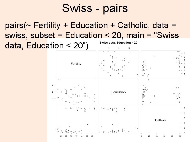
Swiss - pairs(~ Fertility + Education + Catholic, data = swiss, subset = Education < 20, main = "Swiss data, Education < 20") 7

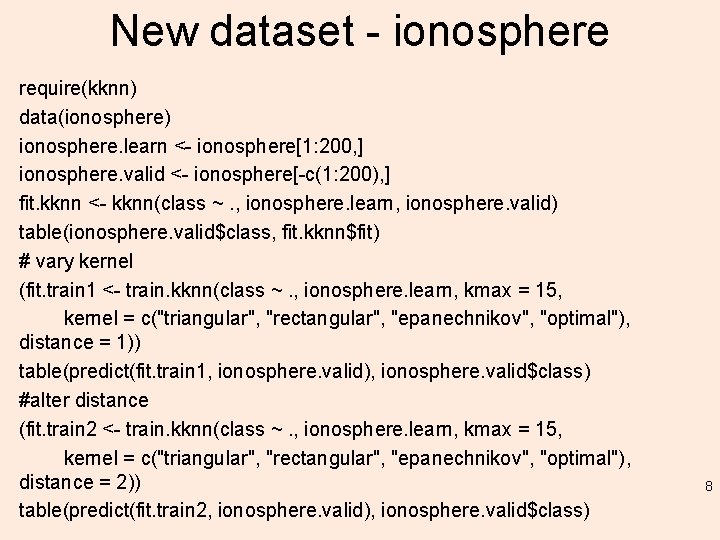
New dataset - ionosphere require(kknn) data(ionosphere) ionosphere. learn <- ionosphere[1: 200, ] ionosphere. valid <- ionosphere[-c(1: 200), ] fit. kknn <- kknn(class ~. , ionosphere. learn, ionosphere. valid) table(ionosphere. valid$class, fit. kknn$fit) # vary kernel (fit. train 1 <- train. kknn(class ~. , ionosphere. learn, kmax = 15, kernel = c("triangular", "rectangular", "epanechnikov", "optimal"), distance = 1)) table(predict(fit. train 1, ionosphere. valid), ionosphere. valid$class) #alter distance (fit. train 2 <- train. kknn(class ~. , ionosphere. learn, kmax = 15, kernel = c("triangular", "rectangular", "epanechnikov", "optimal"), distance = 2)) table(predict(fit. train 2, ionosphere. valid), ionosphere. valid$class) 8

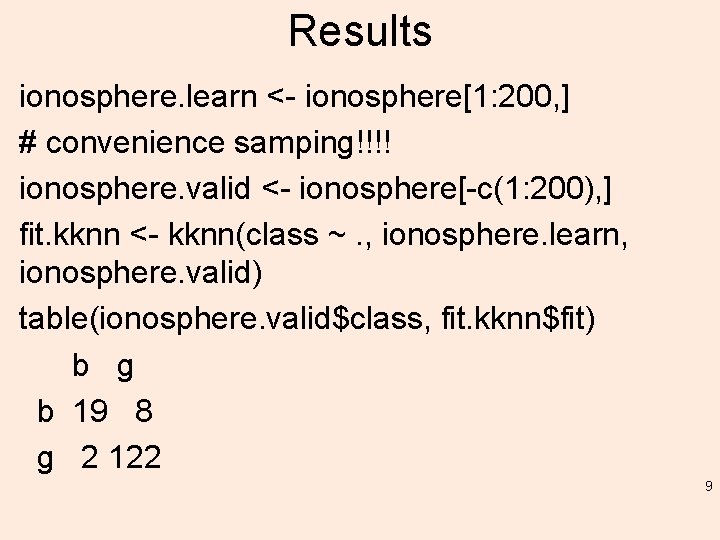
Results ionosphere. learn <- ionosphere[1: 200, ] # convenience samping!!!! ionosphere. valid <- ionosphere[-c(1: 200), ] fit. kknn <- kknn(class ~. , ionosphere. learn, ionosphere. valid) table(ionosphere. valid$class, fit. kknn$fit) b g b 19 8 g 2 122 9

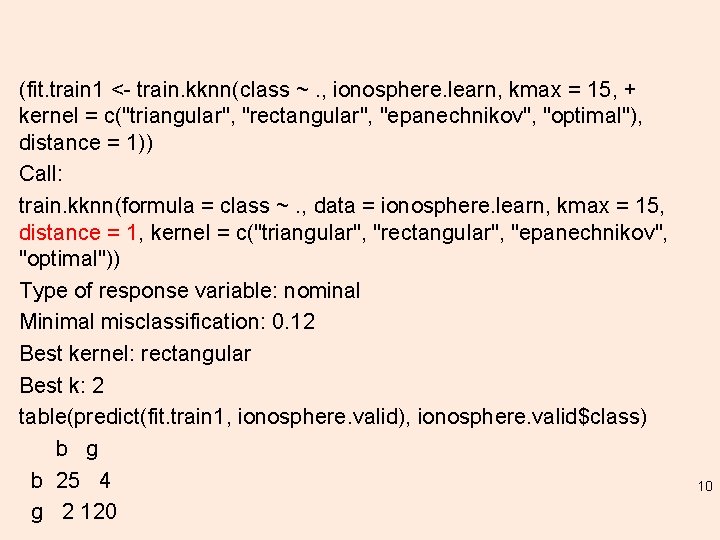
(fit. train 1 <- train. kknn(class ~. , ionosphere. learn, kmax = 15, + kernel = c("triangular", "rectangular", "epanechnikov", "optimal"), distance = 1)) Call: train. kknn(formula = class ~. , data = ionosphere. learn, kmax = 15, distance = 1, kernel = c("triangular", "rectangular", "epanechnikov", "optimal")) Type of response variable: nominal Minimal misclassification: 0. 12 Best kernel: rectangular Best k: 2 table(predict(fit. train 1, ionosphere. valid), ionosphere. valid$class) b g b 25 4 g 2 120 10

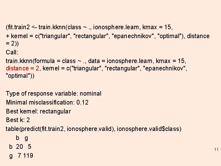
(fit. train 2 <- train. kknn(class ~. , ionosphere. learn, kmax = 15, + kernel = c("triangular", "rectangular", "epanechnikov", "optimal"), distance = 2)) Call: train. kknn(formula = class ~. , data = ionosphere. learn, kmax = 15, distance = 2, kernel = c("triangular", "rectangular", "epanechnikov", "optimal")) Type of response variable: nominal Minimal misclassification: 0. 12 Best kernel: rectangular Best k: 2 table(predict(fit. train 2, ionosphere. valid), ionosphere. valid$class) b g b 20 5 g 7 119 11

However… there is more 12

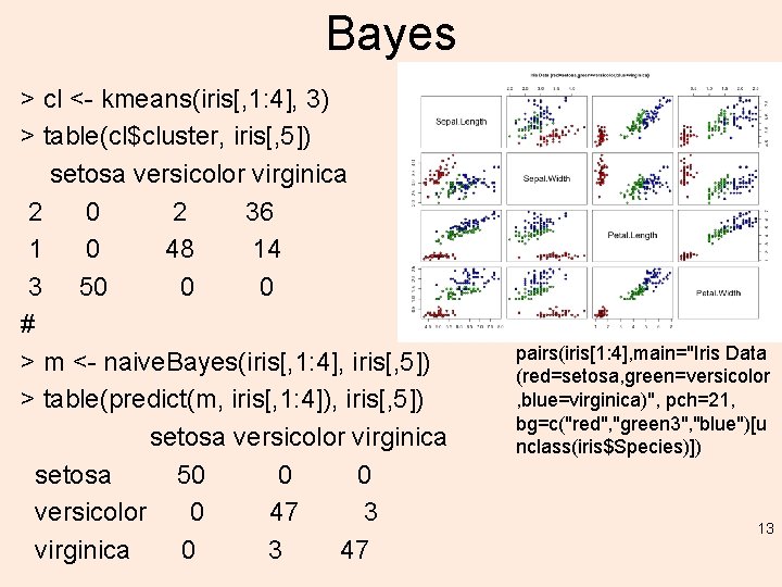
Bayes > cl <- kmeans(iris[, 1: 4], 3) > table(cl$cluster, iris[, 5]) setosa versicolor virginica 2 0 2 36 1 0 48 14 3 50 0 0 # > m <- naive. Bayes(iris[, 1: 4], iris[, 5]) > table(predict(m, iris[, 1: 4]), iris[, 5]) setosa versicolor virginica setosa 50 0 0 versicolor 0 47 3 virginica 0 3 47 pairs(iris[1: 4], main="Iris Data (red=setosa, green=versicolor , blue=virginica)", pch=21, bg=c("red", "green 3", "blue")[u nclass(iris$Species)]) 13

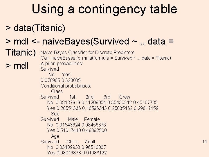
Using a contingency table > data(Titanic) > mdl <- naive. Bayes(Survived ~. , data = Bayes Classifier for Discrete Predictors Titanic) Naive Call: naive. Bayes. formula(formula = Survived ~. , data = Titanic) probabilities: > mdl A-priori Survived No Yes 0. 676965 0. 323035 Conditional probabilities: Class Survived 1 st 2 nd 3 rd Crew No 0. 08187919 0. 11208054 0. 35436242 0. 45167785 Yes 0. 28551336 0. 16596343 0. 25035162 0. 29817159 Sex Survived Male Female No 0. 91543624 0. 08456376 Yes 0. 51617440 0. 48382560 Age Survived Child Adult No 0. 03489933 0. 96510067 Yes 0. 08016878 0. 91983122 14

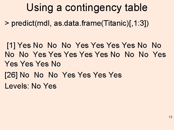
Using a contingency table > predict(mdl, as. data. frame(Titanic)[, 1: 3]) [1] Yes No No No Yes Yes Yes No No No Yes Yes No [26] No No No Yes Yes Levels: No Yes 15

Naïve Bayes – what is it? • Example: testing for a specific item of knowledge that 1% of the population has been informed of (don’t ask how). • An imperfect test: – 99% of knowledgeable people test positive – 99% of ignorant people test negative • If a person tests positive – what is the probability that they know the fact? 16

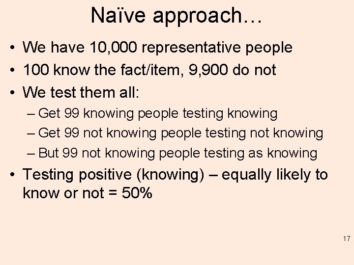
Naïve approach… • We have 10, 000 representative people • 100 know the fact/item, 9, 900 do not • We test them all: – Get 99 knowing people testing knowing – Get 99 not knowing people testing not knowing – But 99 not knowing people testing as knowing • Testing positive (knowing) – equally likely to know or not = 50% 17

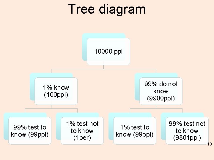
Tree diagram 10000 ppl 1% know (100 ppl) 99% test to know (99 ppl) 1% test not to know (1 per) 99% do not know (9900 ppl) 1% test to know (99 ppl) 99% test not to know (9801 ppl) 18

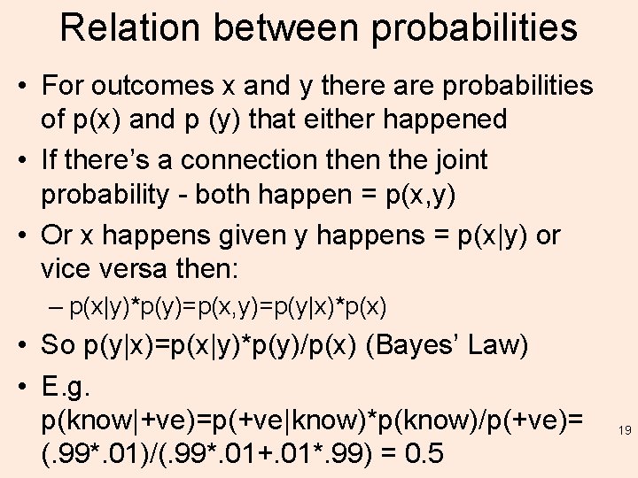
Relation between probabilities • For outcomes x and y there are probabilities of p(x) and p (y) that either happened • If there’s a connection the joint probability - both happen = p(x, y) • Or x happens given y happens = p(x|y) or vice versa then: – p(x|y)*p(y)=p(x, y)=p(y|x)*p(x) • So p(y|x)=p(x|y)*p(y)/p(x) (Bayes’ Law) • E. g. p(know|+ve)=p(+ve|know)*p(know)/p(+ve)= (. 99*. 01)/(. 99*. 01+. 01*. 99) = 0. 5 19

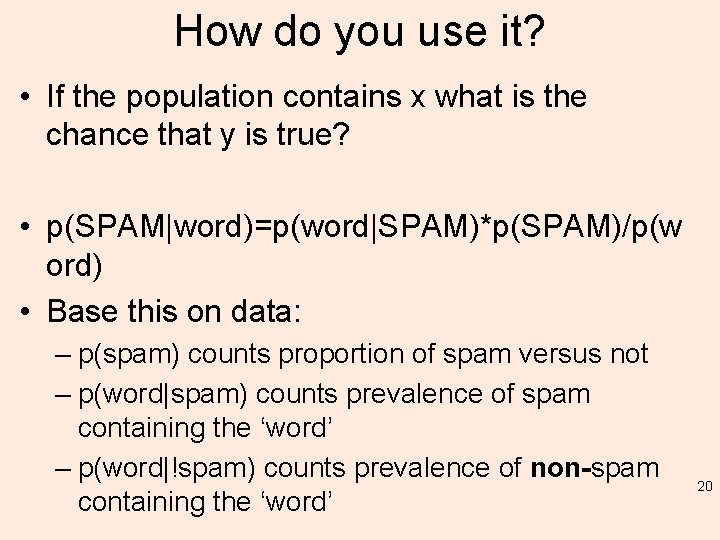
How do you use it? • If the population contains x what is the chance that y is true? • p(SPAM|word)=p(word|SPAM)*p(SPAM)/p(w ord) • Base this on data: – p(spam) counts proportion of spam versus not – p(word|spam) counts prevalence of spam containing the ‘word’ – p(word|!spam) counts prevalence of non-spam containing the ‘word’ 20

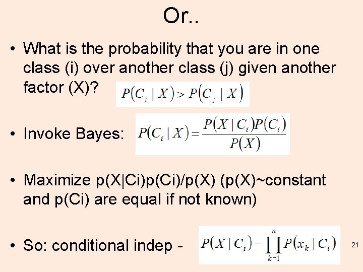
Or. . • What is the probability that you are in one class (i) over another class (j) given another factor (X)? • Invoke Bayes: • Maximize p(X|Ci)p(Ci)/p(X) (p(X)~constant and p(Ci) are equal if not known) • So: conditional indep - 21

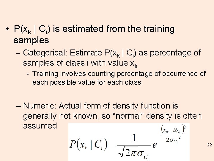
• P(xk | Ci) is estimated from the training samples – Categorical: Estimate P(xk | Ci) as percentage of samples of class i with value xk • Training involves counting percentage of occurrence of each possible value for each class – Numeric: Actual form of density function is generally not known, so “normal” density is often assumed 22

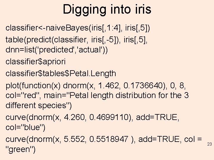
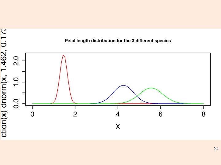
Digging into iris classifier<-naive. Bayes(iris[, 1: 4], iris[, 5]) table(predict(classifier, iris[, -5]), iris[, 5], dnn=list('predicted', 'actual')) classifier$apriori classifier$tables$Petal. Length plot(function(x) dnorm(x, 1. 462, 0. 1736640), 0, 8, col="red", main="Petal length distribution for the 3 different species") curve(dnorm(x, 4. 260, 0. 4699110), add=TRUE, col="blue") curve(dnorm(x, 5. 552, 0. 5518947 ), add=TRUE, col = "green") 23

24

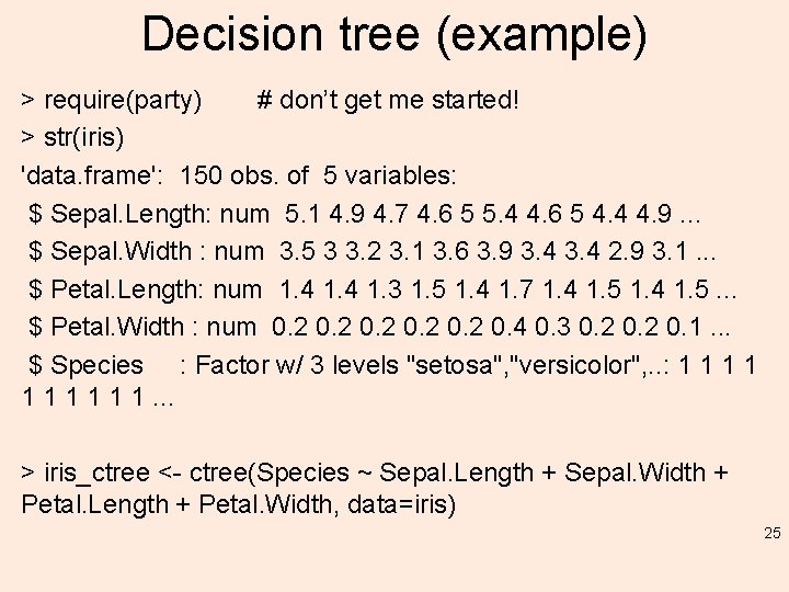
Decision tree (example) > require(party) # don’t get me started! > str(iris) 'data. frame': 150 obs. of 5 variables: $ Sepal. Length: num 5. 1 4. 9 4. 7 4. 6 5 5. 4 4. 6 5 4. 4 4. 9. . . $ Sepal. Width : num 3. 5 3 3. 2 3. 1 3. 6 3. 9 3. 4 2. 9 3. 1. . . $ Petal. Length: num 1. 4 1. 3 1. 5 1. 4 1. 7 1. 4 1. 5. . . $ Petal. Width : num 0. 2 0. 4 0. 3 0. 2 0. 1. . . $ Species : Factor w/ 3 levels "setosa", "versicolor", . . : 1 1 1 1 1. . . > iris_ctree <- ctree(Species ~ Sepal. Length + Sepal. Width + Petal. Length + Petal. Width, data=iris) 25

plot(iris_ctree) 26 > plot(iris_ctree, type="simple”) # try this Try Lab 6 b_5_2014. R

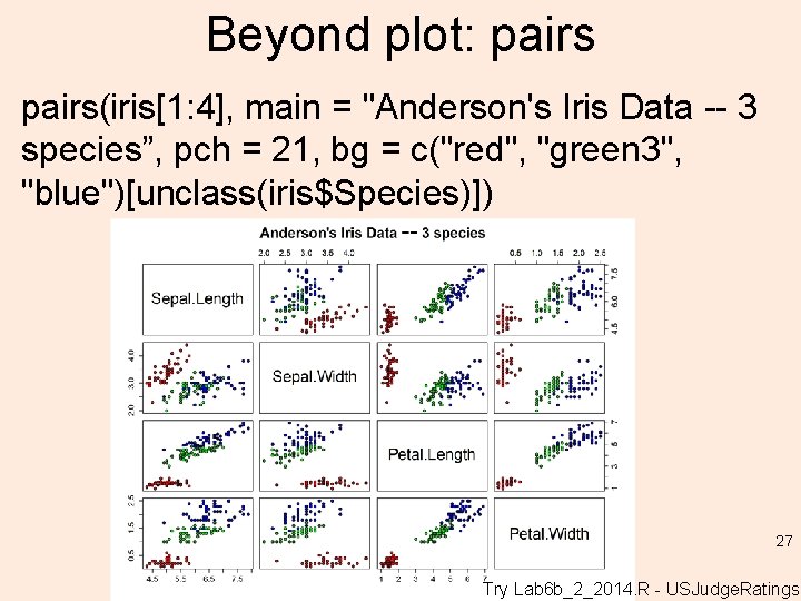
Beyond plot: pairs(iris[1: 4], main = "Anderson's Iris Data -- 3 species”, pch = 21, bg = c("red", "green 3", "blue")[unclass(iris$Species)]) 27 Try Lab 6 b_2_2014. R - USJudge. Ratings

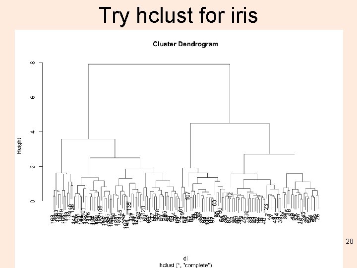
Try hclust for iris 28

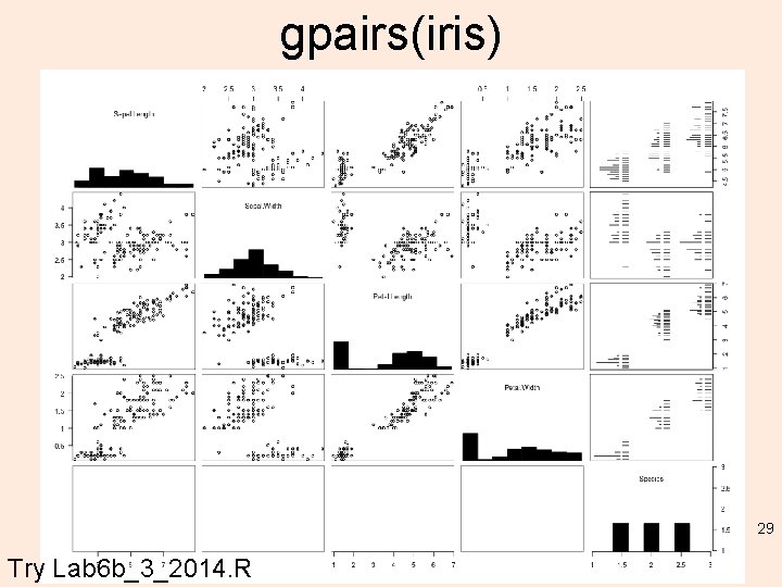
gpairs(iris) 29 Try Lab 6 b_3_2014. R

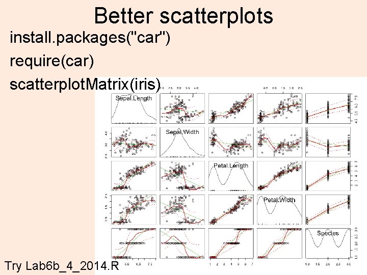
Better scatterplots install. packages("car") require(car) scatterplot. Matrix(iris) 30 Try Lab 6 b_4_2014. R

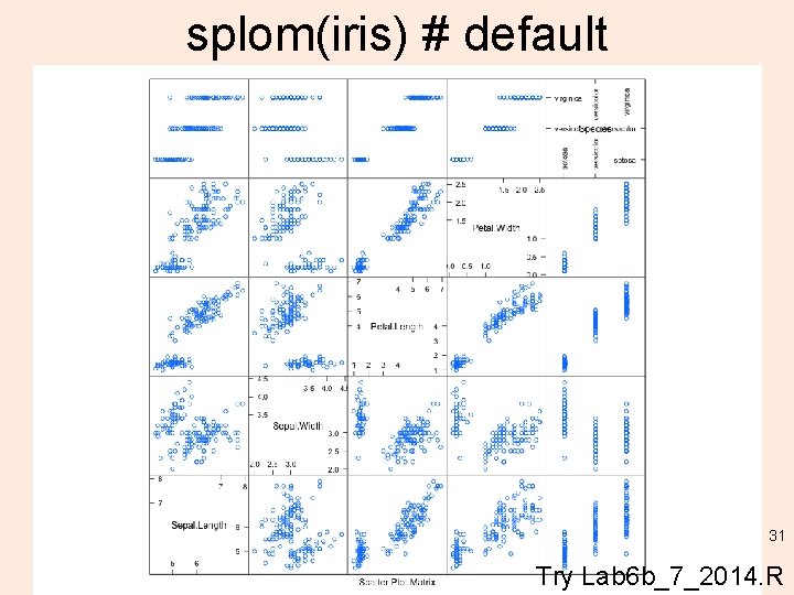
splom(iris) # default 31 Try Lab 6 b_7_2014. R

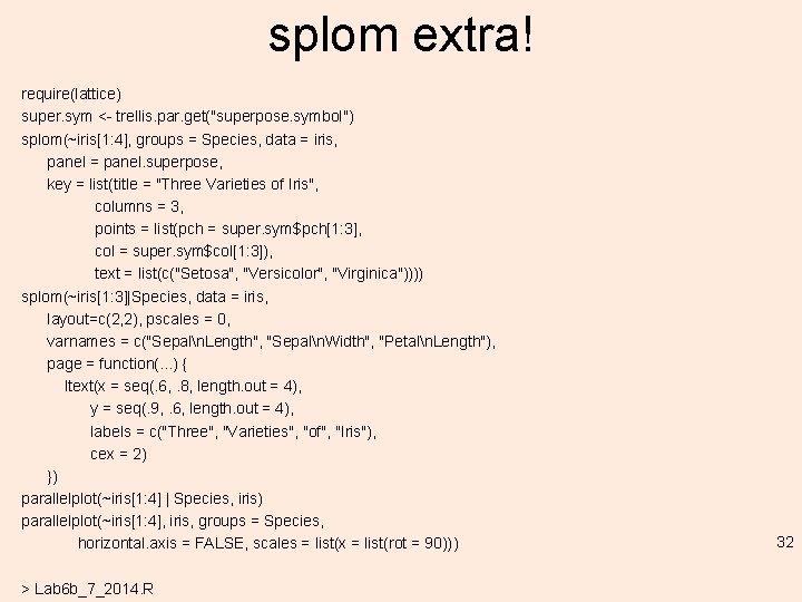
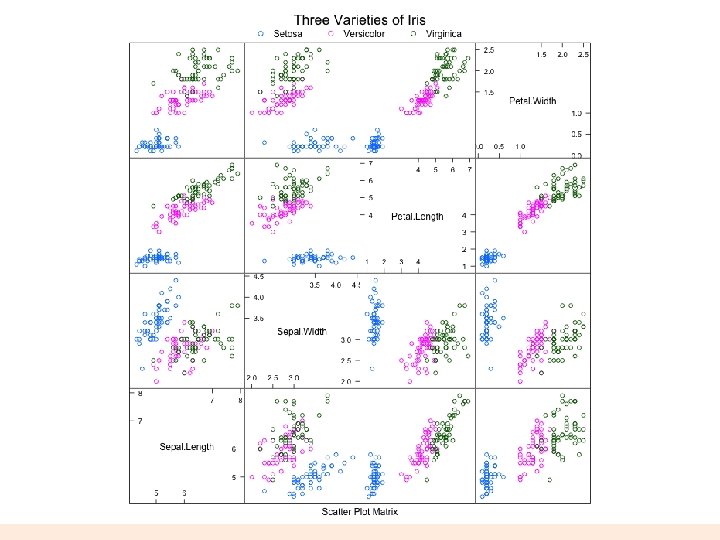
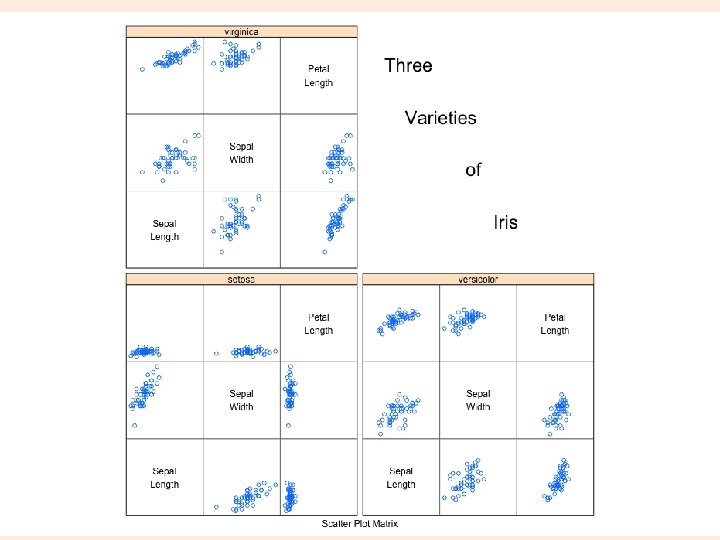
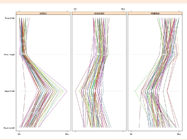
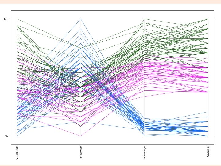
splom extra! require(lattice) super. sym <- trellis. par. get("superpose. symbol") splom(~iris[1: 4], groups = Species, data = iris, panel = panel. superpose, key = list(title = "Three Varieties of Iris", columns = 3, points = list(pch = super. sym$pch[1: 3], col = super. sym$col[1: 3]), text = list(c("Setosa", "Versicolor", "Virginica")))) splom(~iris[1: 3]|Species, data = iris, layout=c(2, 2), pscales = 0, varnames = c("Sepaln. Length", "Sepaln. Width", "Petaln. Length"), page = function(. . . ) { ltext(x = seq(. 6, . 8, length. out = 4), y = seq(. 9, . 6, length. out = 4), labels = c("Three", "Varieties", "of", "Iris"), cex = 2) }) parallelplot(~iris[1: 4] | Species, iris) parallelplot(~iris[1: 4], iris, groups = Species, horizontal. axis = FALSE, scales = list(x = list(rot = 90))) > Lab 6 b_7_2014. R 32

33

34

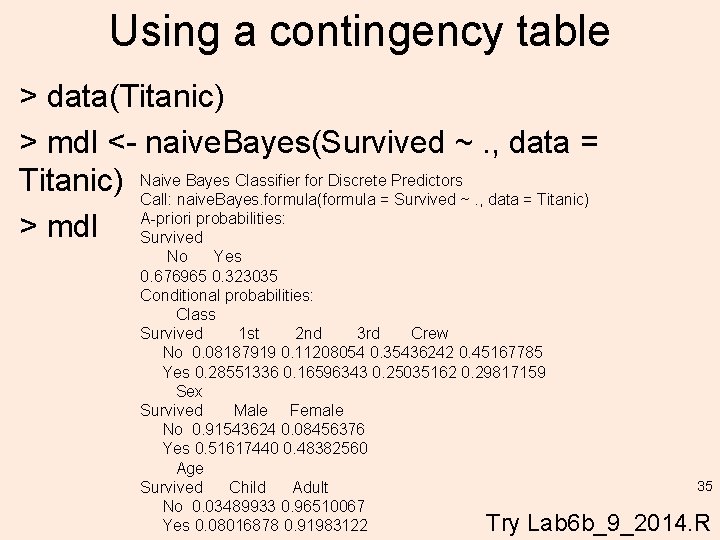
Using a contingency table > data(Titanic) > mdl <- naive. Bayes(Survived ~. , data = Bayes Classifier for Discrete Predictors Titanic) Naive Call: naive. Bayes. formula(formula = Survived ~. , data = Titanic) probabilities: > mdl A-priori Survived No Yes 0. 676965 0. 323035 Conditional probabilities: Class Survived 1 st 2 nd 3 rd Crew No 0. 08187919 0. 11208054 0. 35436242 0. 45167785 Yes 0. 28551336 0. 16596343 0. 25035162 0. 29817159 Sex Survived Male Female No 0. 91543624 0. 08456376 Yes 0. 51617440 0. 48382560 Age 35 Survived Child Adult No 0. 03489933 0. 96510067 Try Lab 6 b_9_2014. R Yes 0. 08016878 0. 91983122

http: //www. ugrad. stat. ubc. ca/R/library/mlb ench/html/House. Votes 84. html require(mlbench) data(House. Votes 84) model <- naive. Bayes(Class ~. , data = House. Votes 84) predict(model, House. Votes 84[1: 10, -1], type = "raw") pred <- predict(model, House. Votes 84[, -1]) table(pred, House. Votes 84$Class) 36

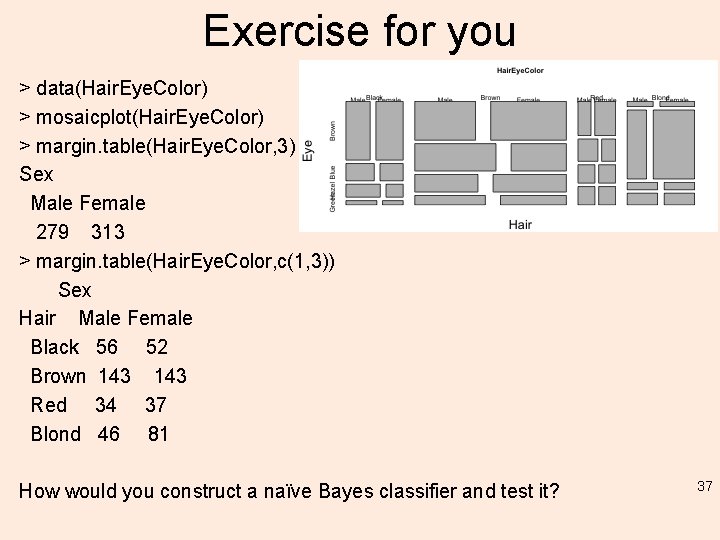
Exercise for you > data(Hair. Eye. Color) > mosaicplot(Hair. Eye. Color) > margin. table(Hair. Eye. Color, 3) Sex Male Female 279 313 > margin. table(Hair. Eye. Color, c(1, 3)) Sex Hair Male Female Black 56 52 Brown 143 Red 34 37 Blond 46 81 How would you construct a naïve Bayes classifier and test it? 37

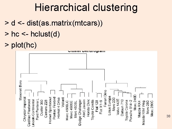
Hierarchical clustering > d <- dist(as. matrix(mtcars)) > hc <- hclust(d) > plot(hc) 38

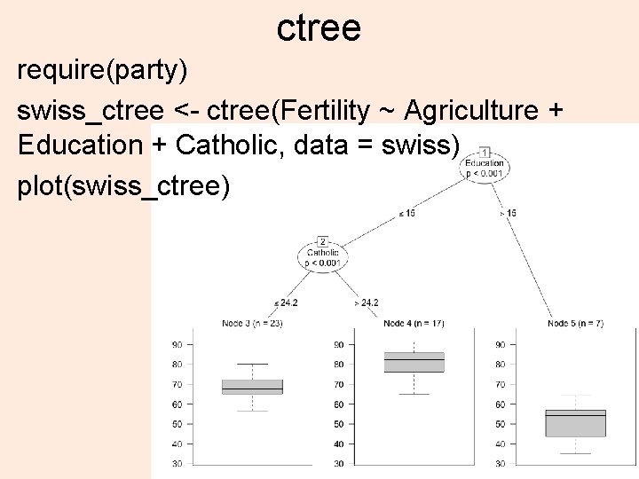
ctree require(party) swiss_ctree <- ctree(Fertility ~ Agriculture + Education + Catholic, data = swiss) plot(swiss_ctree) 39

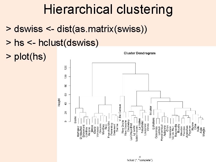
Hierarchical clustering > dswiss <- dist(as. matrix(swiss)) > hs <- hclust(dswiss) > plot(hs) 40

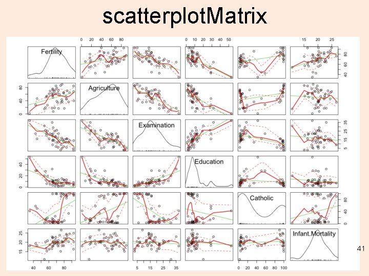
scatterplot. Matrix 41

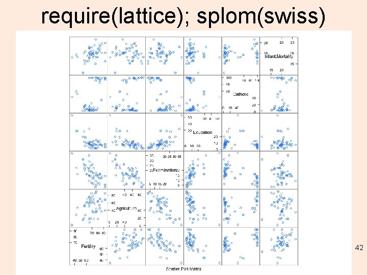
require(lattice); splom(swiss) 42

43

44

At this point… • You may realize the inter-relation among classification at an absolute and relative level (i. e. hierarchical -> trees…) – Trees are interesting from a decision perspective: if this or that, then this…. • Beyond just distance measures (kmeans) to probabilities (Bayesian) • So many ways to visualize them… 45