Weighted graphs Example Consider the following graph where

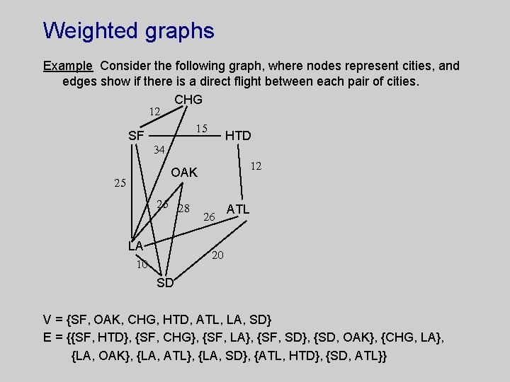
Weighted graphs Example Consider the following graph, where nodes represent cities, and edges show if there is a direct flight between each pair of cities. CHG 12 SF 15 HTD 34 12 OAK 25 25 28 LA 26 ATL 20 10 SD V = {SF, OAK, CHG, HTD, ATL, LA, SD} E = {{SF, HTD}, {SF, CHG}, {SF, LA}, {SF, SD}, {SD, OAK}, {CHG, LA}, {LA, OAK}, {LA, ATL}, {LA, SD}, {ATL, HTD}, {SD, ATL}}

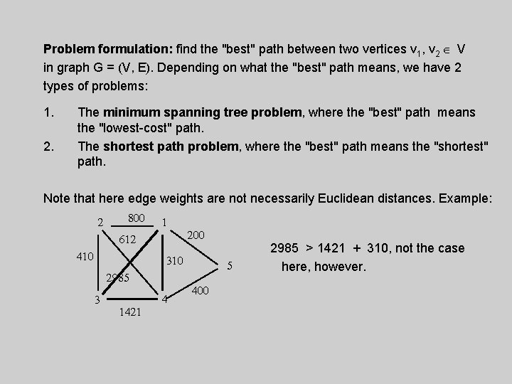
Problem formulation: find the "best" path between two vertices v 1, v 2 V in graph G = (V, E). Depending on what the "best" path means, we have 2 types of problems: 1. 2. The minimum spanning tree problem, where the "best" path means the "lowest-cost" path. The shortest path problem, where the "best" path means the "shortest" path. Note that here edge weights are not necessarily Euclidean distances. Example: 2 800 1 612 410 200 310 2985 3 1421 4 5 400 2985 > 1421 + 310, not the case here, however.

The Weighted Graph ADT Definition A weighted graph, G, is a triple (V, E, W), where (V, E) is a graph, and W is a function from E into Z+, where Z+ is a set of all positive integers. That is, W : E Z+. Additional operations (methods) on weighted graphs: add. Edge(v 1, v 2, weight) Returns G with new edge v 1 v 2 added remove. Edge(v 1, v 2, weight) Returns G with edge v 1 v 2 removed edge. Weight(v 1, v 2) Returns the weight of edge v 1 v 2

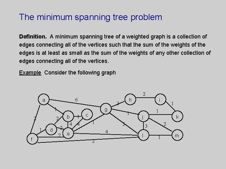
The minimum spanning tree problem Definition. A minimum spanning tree of a weighted graph is a collection of edges connecting all of the vertices such that the sum of the weights of the edges is at least as small as the sum of the weights of any other collection of edges connecting all of the vertices. Example Consider the following graph 2 6 a 1 2 f g 2 1 d h 3 b 4 2 2 e 1 4 1 c 1 1 1 j 5 4 2 i k 2 3 l 1 m

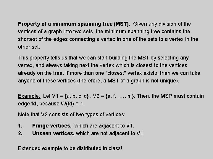
Property of a minimum spanning tree (MST). Given any division of the vertices of a graph into two sets, the minimum spanning tree contains the shortest of the edges connecting a vertex in one of the sets to a vertex in the other set. This property tells us that we can start building the MST by selecting any vertex, and always taking next the vertex which is closest to the vertices already on the tree. If more than one "closest" vertex exists, then we can take anyone of these vertices (therefore, a MST of a graph is not unique). Example: Let V 1 = {a, b, c, d} , V 2 = {e, f, …, m}. Then, the MSP must contain edge fd, because W(fd) = 1. Note that V 2 consists of two types of vertices: 1. 2. Fringe vertices, which are adjacent to V 1. Unseen vertices, which are not adjacent to V 1. Extended example to be distributed in class!

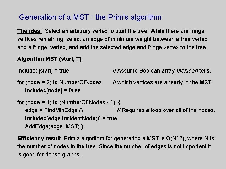
Generation of a MST : the Prim's algorithm The idea: Select an arbitrary vertex to start the tree. While there are fringe vertices remaining, select an edge of minimum weight between a tree vertex and a fringe vertex, and add the selected edge and fringe vertex to the tree. Algorithm MST (start, T) Included[start] = true // Assume Boolean array Included tells, for (node = 2) to Number. Of. Nodes Included[node] = false // which vertices are already in the MST. for (node = 1) to (Number. Of Nodes - 1) { edge = Find. Min. Edge () // Requires a loop over all of the nodes. Included[edge. Incident. Node()] = true Add. Edge(edge, MST) } Efficiency result: Prim's algorithm for generating a MST is O(N^2), where N is the number of nodes in the tree. Since the number of edges is not important it is good for dense graphs.

Generation of a MST : the Kruskal's algorithm The idea: Add edges one at a time selecting at each step the shortest edge that does not form a cycle. Assume that vertices of a MST are initially viewed as one element sets, and edges are arranged in a priority queue according to their weights. Then, we remove edges from the priority queue in order of increasing weights and check if the vertices incident to that edge are already connected. If not, we connect them and this way the disconnected components gradually evolve into a tree -- the minimum spanning tree. Extended example to be distributed in class!

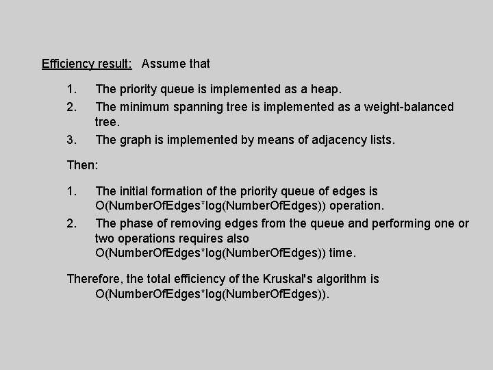
Efficiency result: Assume that 1. 2. 3. The priority queue is implemented as a heap. The minimum spanning tree is implemented as a weight-balanced tree. The graph is implemented by means of adjacency lists. Then: 1. 2. The initial formation of the priority queue of edges is O(Number. Of. Edges*log(Number. Of. Edges)) operation. The phase of removing edges from the queue and performing one or two operations requires also O(Number. Of. Edges*log(Number. Of. Edges)) time. Therefore, the total efficiency of the Kruskal's algorithm is O(Number. Of. Edges*log(Number. Of. Edges)).

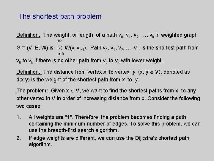
The shortest-path problem Definition. The weight, or length, of a path v 0, v 1, v 2, …, vk in weighted graph k-1 G = (V, E, W) is W(vi vi+1). Path v 0, v 1, v 2, …, vk is the shortest path from i=0 v 0 to vk if there is no other path from v 0 to vk with lower weight. Definition. The distance from vertex x to vertex y (x, y V), denoted as d(x, y) is the weight of the shortest path from x to y. The problem: Given x V, we want to find the shortest paths from x to any other vertex in V in order of increasing distance from x. Consider the following two cases: 1. 2. All weights are "1". Therefore, the problem becomes finding a path containing the minimum number of edges. To solve this problem, we can use the breadth-first search algorithm. If edge weights are different, we can use the Dijkstra's shortest path algorithm.

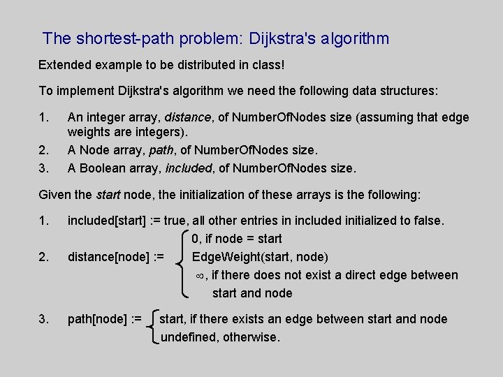
The shortest-path problem: Dijkstra's algorithm Extended example to be distributed in class! To implement Dijkstra's algorithm we need the following data structures: 1. 2. 3. An integer array, distance, of Number. Of. Nodes size (assuming that edge weights are integers). A Node array, path, of Number. Of. Nodes size. A Boolean array, included, of Number. Of. Nodes size. Given the start node, the initialization of these arrays is the following: 1. 2. included[start] : = true, all other entries in included initialized to false. 0, if node = start distance[node] : = Edge. Weight(start, node) , if there does not exist a direct edge between start and node 3. path[node] : = start, if there exists an edge between start and node undefined, otherwise.

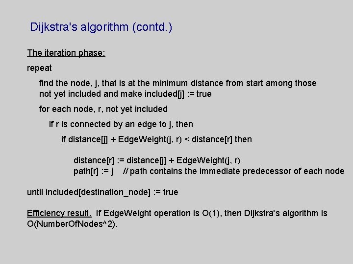
Dijkstra's algorithm (contd. ) The iteration phase: repeat find the node, j, that is at the minimum distance from start among those not yet included and make included[j] : = true for each node, r, not yet included if r is connected by an edge to j, then if distance[j] + Edge. Weight(j, r) < distance[r] then distance[r] : = distance[j] + Edge. Weight(j, r) path[r] : = j // path contains the immediate predecessor of each node until included[destination_node] : = true Efficiency result. If Edge. Weight operation is O(1), then Dijkstra's algorithm is O(Number. Of. Nodes^2).