Week 5 a 1 Lecture 5 a Review

Week 5 a 1

Lecture 5 a Review: Types of Circuit Excitation Why Sinusoidal Excitation? Phasors Week 5 a 2

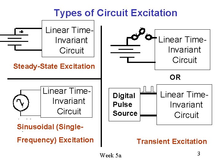
Types of Circuit Excitation Linear Time. Invariant Circuit Steady-State Excitation OR Linear Time. Invariant Circuit Digital Pulse Source Linear Time. Invariant Circuit Sinusoidal (Single. Frequency) Excitation Transient Excitation Week 5 a 3

Why is Sinusoidal Single-Frequency Excitation Important? 1. Some circuits are driven by a single-frequency sinusoidal source. Example: The electric power system at frequency of 60+/-0. 1 Hz in U. S. Voltage is a sinusoidal function of time because it is produced by huge rotating generators powered by mechanical energy source such as steam (produced by heat from natural gas, fuel oil, coal or nuclear fission) or by falling water from a dam (hydroelectric). Week 5 a 4

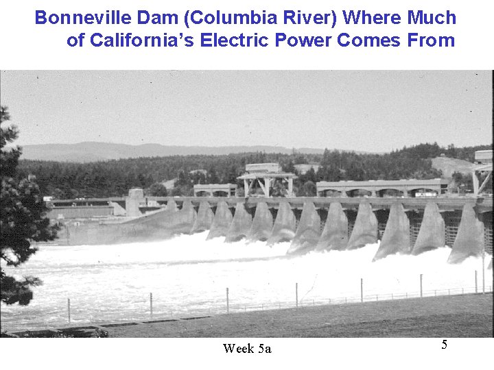
Bonneville Dam (Columbia River) Where Much of California’s Electric Power Comes From Week 5 a 5

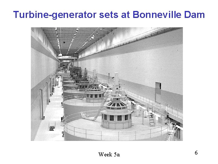
Turbine-generator sets at Bonneville Dam Week 5 a 6

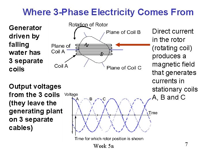
Where 3 -Phase Electricity Comes From Generator driven by falling water has 3 separate coils Direct current in the rotor (rotating coil) produces a magnetic field that generates currents in stationary coils A, B and C Output voltages from the 3 coils (they leave the generating plant on 3 separate cables) Week 5 a 7

Why Sinusoidal Excitation? (continued) 2. Some circuits are driven by sinusoidal sources whose frequency changes slowly over time. 3. Example: Music reproduction system (different notes). 3. And, you can express any periodic electrical signal as a sum of single-frequency sinusoids – so you can analyze the response of the (linear, time-invariant) circuit to each individual frequency component and then sum the responses to get the total response. Week 5 a 8

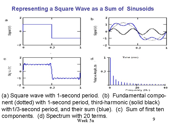
Representing a Square Wave as a Sum of Sinusoids (a) Square wave with 1 -second period. (b) Fundamental component (dotted) with 1 -second period, third-harmonic (solid black) with 1/3 -second period, and their sum (blue). (c) Sum of first ten components. (d) Spectrum with 20 terms. 9 Week 5 a

Single-frequency sinusoidal-excitation AC circuit problems 1. The technique we’ll show works on circuits composed of linear elements (R, C, L) that don’t change with time “linear time-invariant circuits”. 2. The circuit is driven with independent voltage and/or current sources whose voltages or currents vary at a single frequency, f, measured in Hertz (abbreviated Hz) this is the number of cycles the voltages or currents execute per second. We can represent the source voltages or currents as functions of time as v(t) = V 0 cos(wt) or i(t) = I 0 cos(wt), where w = 2 pf is the angular frequency in radians per second. Example: In the U. S. the AC power frequency, f, is 60 Hz and the peak voltage V 0 is 170 V, so w = 377 radians/s and v(t) = 170 cos(377 t) V. More generally, we might have sources v(t) = V 0 sin(wt) or i(t) = I 0 cos(wt = f), where f is a phase angle. Week 5 a 10

We could solve our circuit equations using such functions of time, but we’d have to do a lot of tedious trigonometric transformations. Instead we use a mathematical trick to eliminate time dependence from our equations! The trick is based on a fundamental fact about linear, timeinvariant circuits excited with sinusoidal sources: the frequencies of all the voltages and currents in the circuit are identical. Week 5 a 11

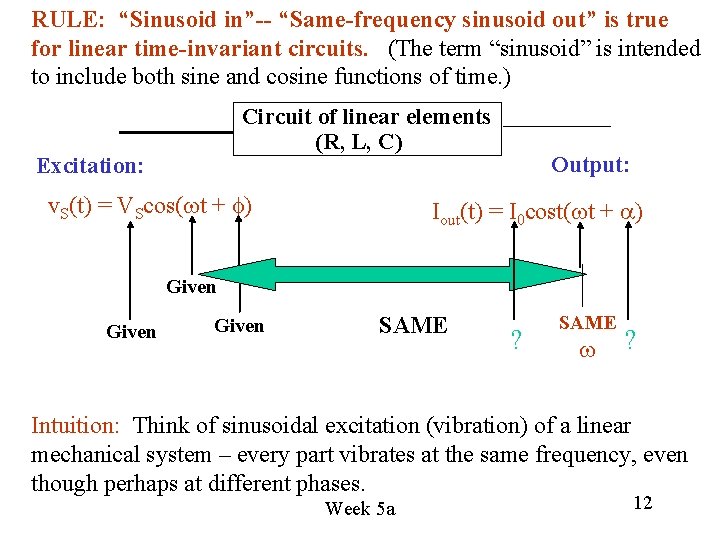
RULE: “Sinusoid in”-- “Same-frequency sinusoid out” is true for linear time-invariant circuits. (The term “sinusoid” is intended to include both sine and cosine functions of time. ) Circuit of linear elements (R, L, C) Excitation: v. S(t) = VScos(wt + f) Output: Iout(t) = I 0 cost(wt + a) Given SAME ? SAME w ? Intuition: Think of sinusoidal excitation (vibration) of a linear mechanical system – every part vibrates at the same frequency, even though perhaps at different phases. Week 5 a 12

You can solve AC circuit analysis problems that involve Circuits with linear elements (R, C, L) plus independent and dependent voltage and/or current sources operating at a single angular frequency w = 2 pf (radians/s) such as v(t) = V 0 cos(wt) or i(t) = I 0 cos(wt). By using any of Ohm’s Law, KVL and KCL equations, doing superposition analysis, nodal analysis or mesh analysis, AND Using instead of the terms below on the left (general excitation), the terms below on the right (sinusoidal excitation): Week 5 a 13

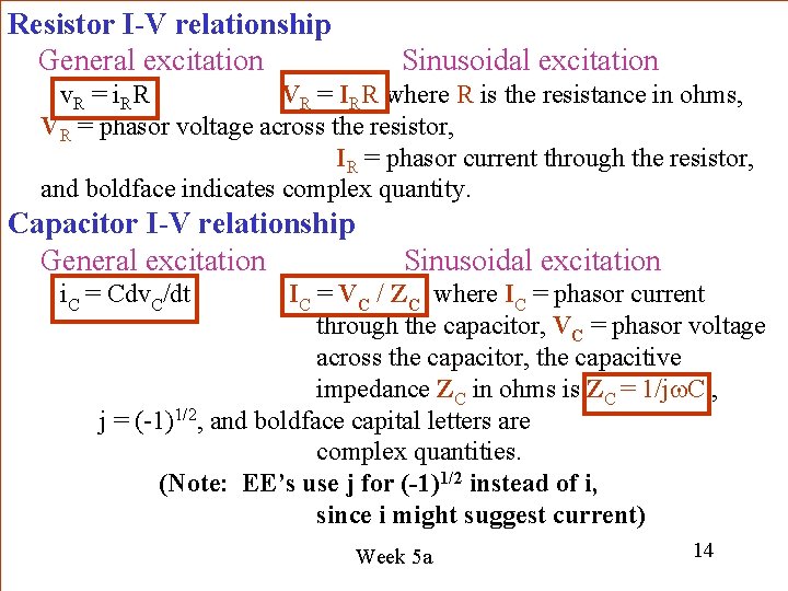
Resistor I-V relationship General excitation Sinusoidal excitation v. R = i. RR VR = IRR where R is the resistance in ohms, VR = phasor voltage across the resistor, IR = phasor current through the resistor, and boldface indicates complex quantity. Capacitor I-V relationship General excitation Sinusoidal excitation i. C = Cdv. C/dt IC = VC / ZC where IC = phasor current through the capacitor, VC = phasor voltage across the capacitor, the capacitive impedance ZC in ohms is ZC = 1/jw. C , j = (-1)1/2, and boldface capital letters are complex quantities. (Note: EE’s use j for (-1)1/2 instead of i, since i might suggest current) Week 5 a 14

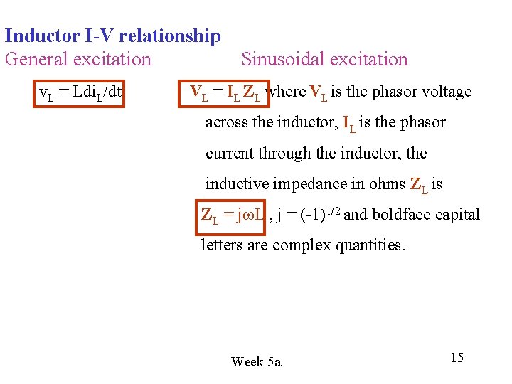
Inductor I-V relationship General excitation Sinusoidal excitation v. L = Ldi. L/dt VL = IL ZL where VL is the phasor voltage across the inductor, IL is the phasor current through the inductor, the inductive impedance in ohms ZL is ZL = jw. L , j = (-1)1/2 and boldface capital letters are complex quantities. Week 5 a 15

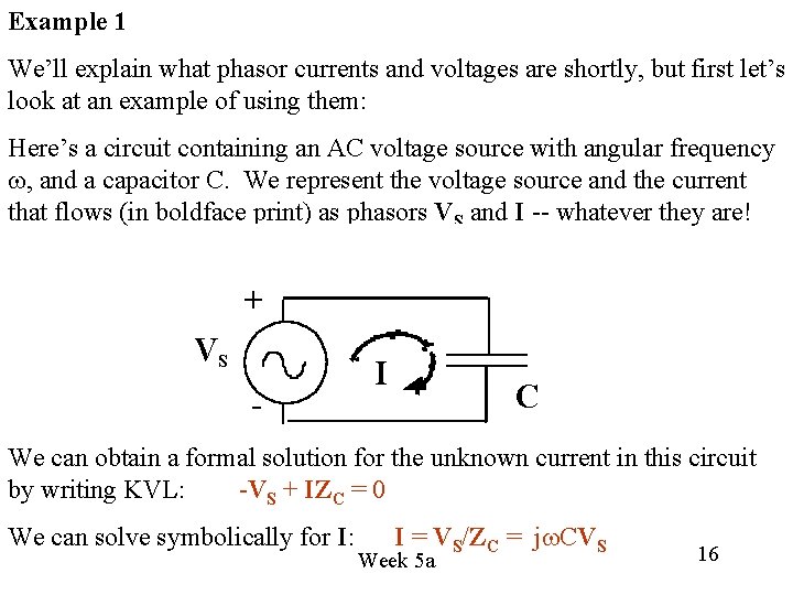
Example 1 We’ll explain what phasor currents and voltages are shortly, but first let’s look at an example of using them: Here’s a circuit containing an AC voltage source with angular frequency w, and a capacitor C. We represent the voltage source and the current that flows (in boldface print) as phasors VS and I -- whatever they are! + VS - I C We can obtain a formal solution for the unknown current in this circuit by writing KVL: -VS + IZC = 0 We can solve symbolically for I: I = VS/ZC = jw. CVS Week 5 a 16

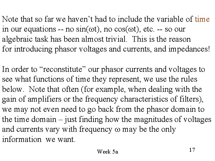
Note that so far we haven’t had to include the variable of time in our equations -- no sin(wt), no cos(wt), etc. -- so our algebraic task has been almost trivial. This is the reason for introducing phasor voltages and currents, and impedances! In order to “reconstitute” our phasor currents and voltages to see what functions of time they represent, we use the rules below. Note that often (for example, when dealing with the gain of amplifiers or the frequency characteristics of filters), we may not even need to go back from the phasor domain to the time domain – just finding how the magnitudes of voltages and currents vary with frequency w may be the only information we want. Week 5 a 17

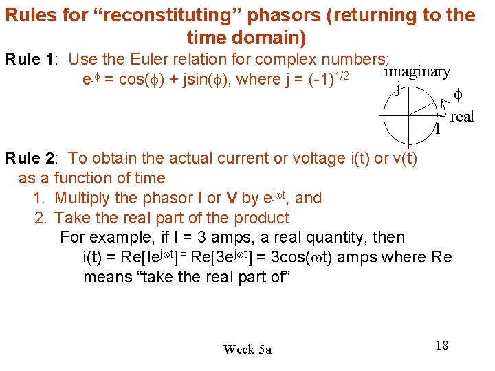
Rules for “reconstituting” phasors (returning to the time domain) Rule 1: Use the Euler relation for complex numbers: imaginary ejf = cos(f) + jsin(f), where j = (-1)1/2 j 1 f real Rule 2: To obtain the actual current or voltage i(t) or v(t) as a function of time 1. Multiply the phasor I or V by ejwt, and 2. Take the real part of the product For example, if I = 3 amps, a real quantity, then i(t) = Re[Iejwt] = Re[3 ejwt] = 3 cos(wt) amps where Re means “take the real part of” Week 5 a 18

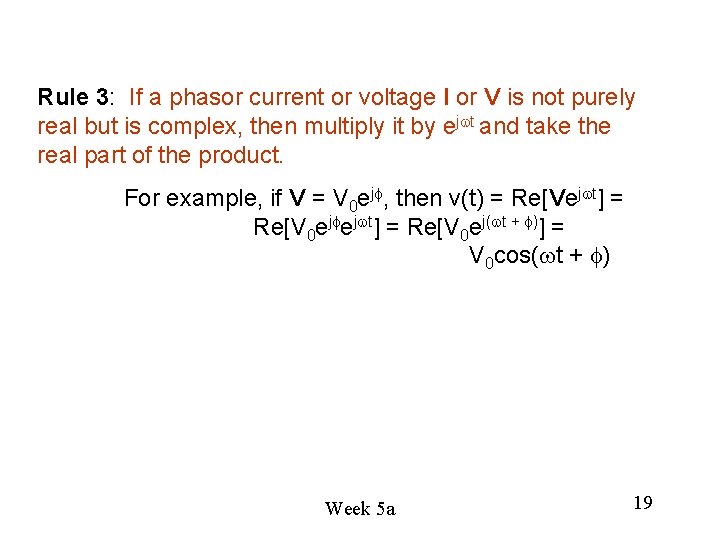
Rule 3: If a phasor current or voltage I or V is not purely real but is complex, then multiply it by ejwt and take the real part of the product. For example, if V = V 0 ejf, then v(t) = Re[Vejwt] = Re[V 0 ejfejwt] = Re[V 0 ej(wt + f)] = V 0 cos(wt + f) Week 5 a 19

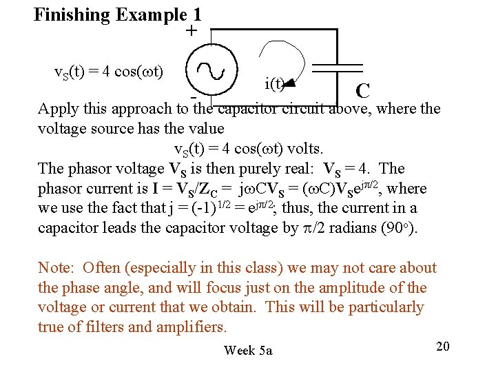
Finishing Example 1 + v. S(t) = 4 cos(wt) - i(t) C Apply this approach to the capacitor circuit above, where the voltage source has the value v. S(t) = 4 cos(wt) volts. The phasor voltage VS is then purely real: VS = 4. The phasor current is I = VS/ZC = jw. CVS = (w. C)VSejp/2, where we use the fact that j = (-1)1/2 = ejp/2; thus, the current in a capacitor leads the capacitor voltage by p/2 radians (90 o). Note: Often (especially in this class) we may not care about the phase angle, and will focus just on the amplitude of the voltage or current that we obtain. This will be particularly true of filters and amplifiers. Week 5 a 20

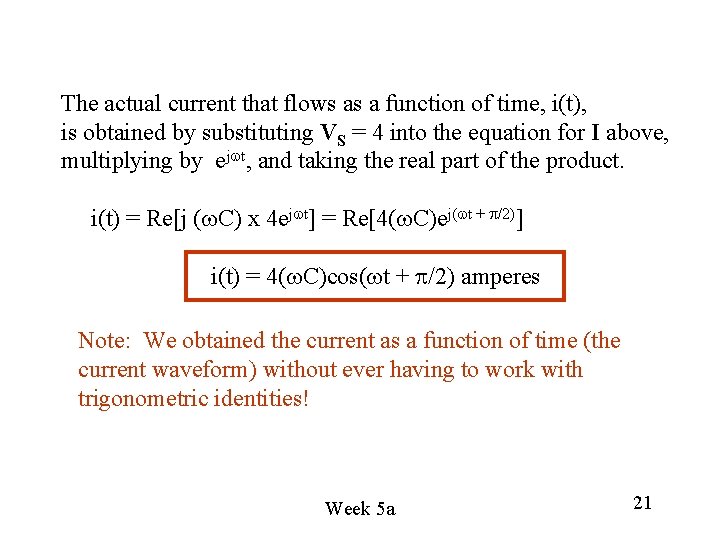
The actual current that flows as a function of time, i(t), is obtained by substituting VS = 4 into the equation for I above, multiplying by ejwt, and taking the real part of the product. i(t) = Re[j (w. C) x 4 ejwt] = Re[4(w. C)ej(wt + p/2)] i(t) = 4(w. C)cos(wt + p/2) amperes Note: We obtained the current as a function of time (the current waveform) without ever having to work with trigonometric identities! Week 5 a 21

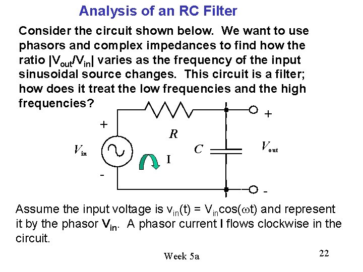
Analysis of an RC Filter Consider the circuit shown below. We want to use phasors and complex impedances to find how the ratio |Vout/Vin| varies as the frequency of the input sinusoidal source changes. This circuit is a filter; how does it treat the low frequencies and the high frequencies? + + R Vout C Vin I Assume the input voltage is vin(t) = Vincos(wt) and represent it by the phasor Vin. A phasor current I flows clockwise in the circuit. Week 5 a 22

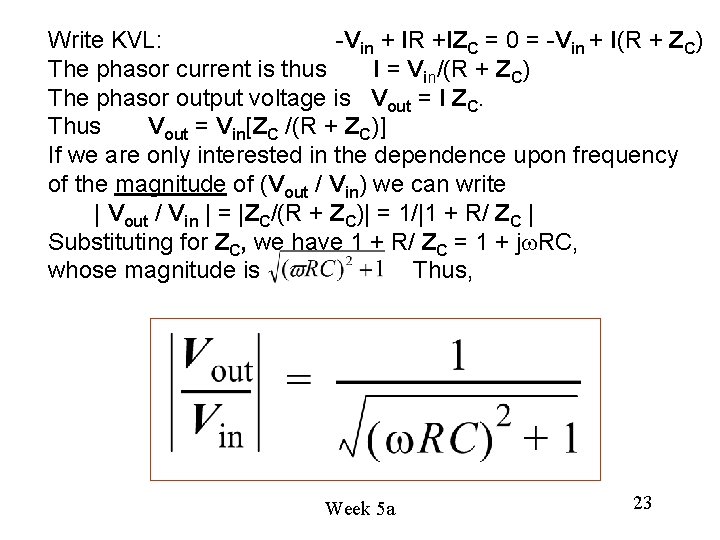
Write KVL: -Vin + IR +IZC = 0 = -Vin + I(R + ZC) The phasor current is thus I = Vin/(R + ZC) The phasor output voltage is Vout = I ZC. Thus Vout = Vin[ZC /(R + ZC)] If we are only interested in the dependence upon frequency of the magnitude of (Vout / Vin) we can write | Vout / Vin | = |ZC/(R + ZC)| = 1/|1 + R/ ZC | Substituting for ZC, we have 1 + R/ ZC = 1 + jw. RC, whose magnitude is Thus, Week 5 a 23

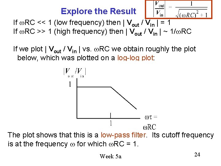
Explore the Result If w. RC << 1 (low frequency) then | Vout / Vin | = 1 If w. RC >> 1 (high frequency) then | Vout / Vin | ~ 1/w. RC If we plot | Vout / Vin | vs. w. RC we obtain roughly the plot below, which was plotted on a log-log plot: The plot shows that this is a low-pass filter. Its cutoff frequency is at the frequency w for which w. RC = 1. Week 5 a 24

Notice that we’ve obtained a lot of information about how this particular RC circuit performs just by looking at the magnitude of the ratio of phasor output voltage to phasor input voltage (i. e. , we haven’t had to study the phase angles associted with those phasor voltages. (In more detailed studies the phase angles can be important – but not in this course. ) Does this behavior make sense from what we know about capacitors? YES! At low frequency a capacitor is like an open circuit – so the output voltage would equal the input voltage At high frequency a capacitor is like a short circuit – so the output voltage would be very small. Week 5 a 25

Here is a useful web site to explore: http: //www. phys. unsw. edu. au/~jw/AC. html You’ll find some demonstrations dealing with phasors and impedances there. And Appendix A in Hambley is a review of complex numbers. Week 5 a 26

Why Does the Phasor Approach Work? 1. Phasors are discussed at length in your text (Hambley 3 rd Ed. , pp. 195 -201) with an interpretation that sinusoids can be visualized as the real axis projection of vectors rotating in the complex plane, as in Fig. 5. 4. This is the most basic connection between sinusoids and phasors. 2. We present phasors as a convenient tool for analysis of linear time-invariant circuits with a sinusoidal excitation. The basic reason for using them is that they eliminate the time dependence in such circuits, greatly simplifying the analysis. 3. Your text discusses complex impedances in Sec. 5. 3, and circuit analysis with phasors and complex impedances in Sec. 5. 4. Skim over this LIGHTLY. Week 5 a 27

Motivations for Including Phasors in EECS 40 1. It enables us to include a lab where you measure the behavior of RC filters as a function of frequency, and use Lab. VIEW to automate that measurement. 2. It enables us to (probably) include a nice operational amplifier lab project near the end of the course to make an “active” filter (the RC filter is passive). 3. It enables you to find out what impedances are and use them as real EEs do. 4. The subject was also supposedly included (in a way) in EECS 20 which some of you may have taken. Week 5 a 28