Week 12 November 17 21 Four MiniLectures QMM

Week 12 November 17 -21 Four Mini-Lectures QMM 510 Fall 2014

ML 12. 1 Chapter Contents 13. 1 Multiple Regression 13. 2 Assessing Overall Fit 13. 3 Predictor Significance 13. 4 Confidence Intervals for Y 13. 5 Categorical Predictors 13. 6 Tests for Nonlinearity and Interaction 13. 7 Multicollinearity 13. 8 Violations of Assumptions 13. 9 Other Regression Topics 13 -2 Much of this is like Chapter 12, except that we have more than one predictor. Chapter 13 Multiple Regression

Chapter 13 Multiple Regression Simple or Multivariate? • Multiple regression is an extension of simple regression to include more than one independent variable. • Limitations of simple regression: • often simplistic • biased estimates if relevant predictors are omitted • lack of fit does not show that X is unrelated to Y if the true model is multivariate 13 -3

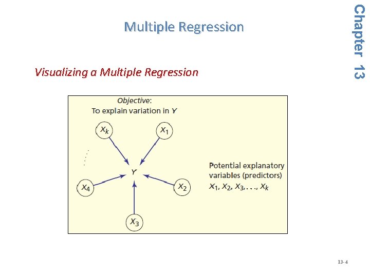
Chapter 13 Multiple Regression Visualizing a Multiple Regression 13 -4

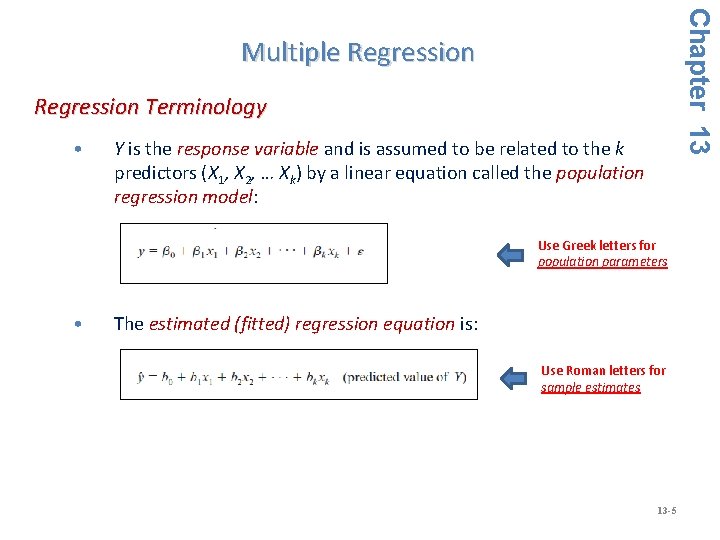
Chapter 13 Multiple Regression Terminology • Y is the response variable and is assumed to be related to the k predictors (X 1, X 2, … Xk) by a linear equation called the population regression model: Use Greek letters for population parameters • The estimated (fitted) regression equation is: Use Roman letters for sample estimates 13 -5

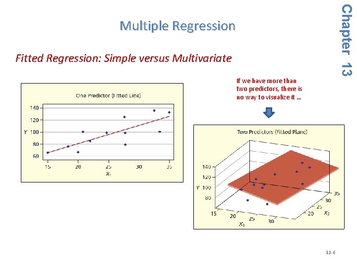
Chapter 13 Multiple Regression Fitted Regression: Simple versus Multivariate If we have more than two predictors, there is no way to visualize it … 13 -6

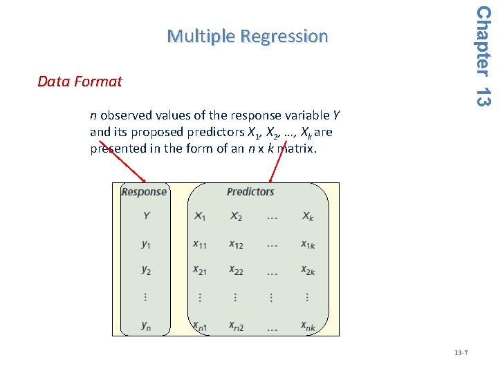
Chapter 13 Multiple Regression Data Format n observed values of the response variable Y and its proposed predictors X 1, X 2, …, Xk are presented in the form of an n x k matrix. 13 -7

Chapter 13 Multiple Regression Common Misconceptions about Fit • A common mistake is to assume that the model with the best fit is preferred. • Sometimes a model with a low R 2 may give useful predictions, while a model with a high R 2 may conceal problems. • Thoroughly analyze the results before choosing the model. 13 -8

Chapter 13 Multiple Regression Four Criteria for Regression Assessment • Logic - Is there an a priori reason to expect a causal relationship between the predictors and the response variable? • Fit - Does the overall regression show a significant relationship between the predictors and the response variable? • Parsimony - Does each predictor contribute significantly to the explanation? Are some predictors not worth the trouble? • Stability - Are the predictors related to one another so strongly that the regression estimates become erratic? 13 -9

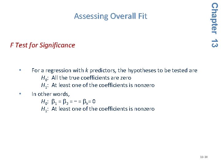
Chapter 13 Assessing Overall Fit F Test for Significance • • For a regression with k predictors, the hypotheses to be tested are H 0: All the true coefficients are zero H 1: At least one of the coefficients is nonzero In other words, H 0 : b 1 = b 2 = … = b k = 0 H 1: At least one of the coefficients is nonzero 13 -10

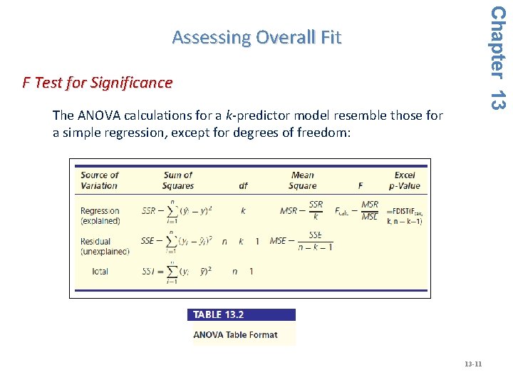
Chapter 13 Assessing Overall Fit F Test for Significance The ANOVA calculations for a k-predictor model resemble those for a simple regression, except for degrees of freedom: 13 -11

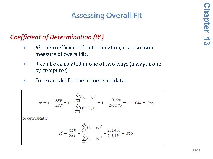
Chapter 13 Assessing Overall Fit Coefficient of Determination (R 2) • R 2, the coefficient of determination, is a common measure of overall fit. • It can be calculated in one of two ways (always done by computer). • For example, for the home price data, 13 -12

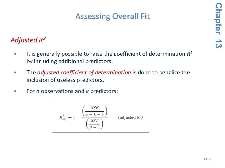
Chapter 13 Assessing Overall Fit Adjusted R 2 • It is generally possible to raise the coefficient of determination R 2 by including additional predictors. • The adjusted coefficient of determination is done to penalize the inclusion of useless predictors. • For n observations and k predictors: 13 -13

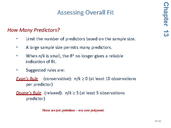
Chapter 13 Assessing Overall Fit How Many Predictors? • Limit the number of predictors based on the sample size. • A large sample size permits many predictors. • When n/k is small, the R 2 no longer gives a reliable indication of fit. • Suggested rules are: Evan’s Rule (conservative): n/k 0 (at least 10 observations per predictor) Doane’s Rule (relaxed): n/k 5 (at least 5 observations predictor) These are just guidelines – use your judgment. 13 -14

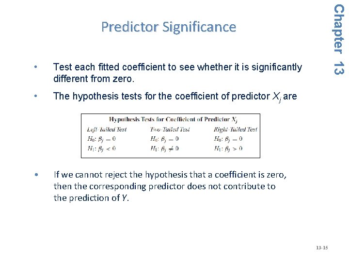
Chapter 13 Predictor Significance • Test each fitted coefficient to see whether it is significantly different from zero. • The hypothesis tests for the coefficient of predictor Xj are • If we cannot reject the hypothesis that a coefficient is zero, then the corresponding predictor does not contribute to the prediction of Y. 13 -15

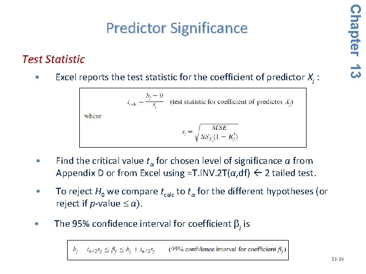
Chapter 13 Predictor Significance Test Statistic • Excel reports the test statistic for the coefficient of predictor Xj : • Find the critical value tα for chosen level of significance α from Appendix D or from Excel using =T. INV. 2 T(α, df) 2 tailed test. • To reject H 0 we compare tcalc to tα for the different hypotheses (or reject if p-value α). • The 95% confidence interval for coefficient bj is 13 -16

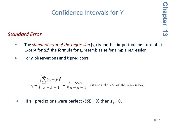
Chapter 13 Confidence Intervals for Y Standard Error • The standard error of the regression (se) is another important measure of fit. Except for d. f. the formula for se resembles se for simple regression. • For n observations and k predictors • If all predictions were perfect (SSE = 0) then se = 0. 13 -17

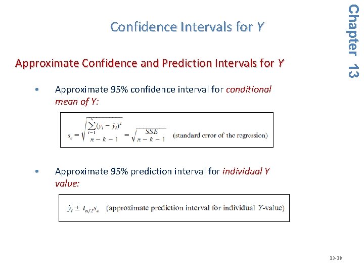
Chapter 13 Confidence Intervals for Y Approximate Confidence and Prediction Intervals for Y • Approximate 95% confidence interval for conditional mean of Y: • Approximate 95% prediction interval for individual Y value: 13 -18

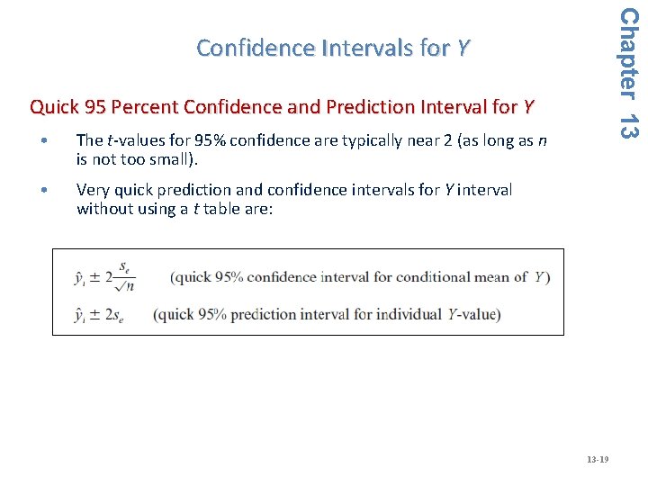
Chapter 13 Confidence Intervals for Y Quick 95 Percent Confidence and Prediction Interval for Y • The t-values for 95% confidence are typically near 2 (as long as n is not too small). • Very quick prediction and confidence intervals for Y interval without using a t table are: 13 -19

ML 12. 2 Standardized Residuals • Use Excel, MINITAB, Mega. Stat or other software to compute standardized residuals. • If the absolute value of any standardized residual is at least 2, then it is classified as unusual (as in simple regression). Leverage and Influence • A high leverage statistic indicates unusual X values in one or more predictors. • Such observations are influential because they are near the edge(s) of the fitted regression plane. • Leverage for observation i is denoted hi (computed by Mega. Stat) 12 -20 Chapter 13 Unusual Observations

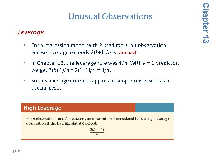
Leverage • For a regression model with k predictors, an observation whose leverage exceeds 2(k+1)/n is unusual • In Chapter 12, the leverage rule was 4/n. With k = 1 predictor, we get 2(k+1)/n = 2(1+1)/n = 4/n. • So this leverage criterion applies to simple regression as a special case. 12 -21 Chapter 13 Unusual Observations

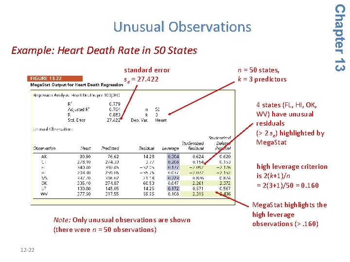
Example: Heart Death Rate in 50 States standard error se = 27. 422 n = 50 states, k = 3 predictors 4 states (FL, HI, OK, WV) have unusual residuals (> 2 se) highlighted by Mega. Stat high leverage criterion is 2(k+1)/n = 2(3+1)/50 = 0. 160 Note: Only unusual observations are shown (there were n = 50 observations) 12 -22 Mega. Stat highlights the high leverage observations (>. 160) Chapter 13 Unusual Observations

Chapter 13 Categorical Predictors ML 12. 3 What Is a Binary or Categorical Predictor? • A binary predictor has two values (usually 0 and 1) to denote the presence or absence of a condition. • For example, for n graduates from an MBA program: Employed = 1 Unemployed = 0 • These variables are also called dummy , dichotomous, or indicator variables. • For easy understandability, name the binary variable the characteristic that is equivalent to the value of 1. 13 -23

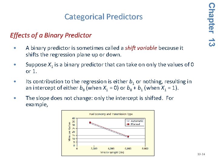
Chapter 13 Categorical Predictors Effects of a Binary Predictor • A binary predictor is sometimes called a shift variable because it shifts the regression plane up or down. • Suppose X 1 is a binary predictor that can take on only the values of 0 or 1. • Its contribution to the regression is either b 1 or nothing, resulting in an intercept of either b 0 (when X 1 = 0) or b 0 + b 1 (when X 1 = 1). • The slope does not change: only the intercept is shifted. For example, 13 -24

Testing a Binary for Significance • In multiple regression, binary predictors require no special treatment. They are tested as any other predictor using a t test. More Than One Binary • More than one binary occurs when the number of categories to be coded exceeds two. • For example, for the variable GPA by class level, each category is a binary variable: Freshman = 1 if a freshman, 0 otherwise Sophomore = 1 if a sophomore, 0 otherwise Junior = 1 if a junior, 0 otherwise Senior = 1 if a senior, 0 otherwise Masters = 1 if a master’s candidate, 0 otherwise Doctoral = 1 if a Ph. D candidate, 0 otherwise 13 -25 Chapter 13 Categorical Predictors

What if I Forget to Exclude One Binary? • Including all binaries for all categories may introduce a serious problem of collinearity for the regression estimation. Collinearity occurs when there are redundant independent variables. • When the value of one independent variable can be determined from the values of other independent variables, one column in the X data matrix will be a perfect linear combination of the other column(s). • The least squares estimation would fail because the data matrix would be singular (i. e. , would have no inverse). 13 -26 Chapter 13 Categorical Predictors

• Outliers? (omit only if clearly errors) • Missing Predictors? (usually you can’t tell) • Ill-Conditioned Data (adjust decimals or take logs) • Significance in Large Samples? (if n is huge, almost any regression will be significant) • Model Specification Errors? (may show up in residual patterns) • Missing Data? (we may have to live without it) • Binary Response? (if Y = 0, 1 we use logistic regression) • Stepwise and Best Subsets Regression (Mega. Stat does these) 13 -27 Chapter 13 Other Regression Problems