Week 11 TCP Congestion Control 1 Principles of

Week 11 TCP Congestion Control 1

Principles of Congestion Control Congestion: r informally: “too many sources sending too much data too fast for network to handle” r different from flow control! r manifestations: m lost packets (buffer overflow at routers) m long delays (queueing in router buffers) r a top-10 problem! 2

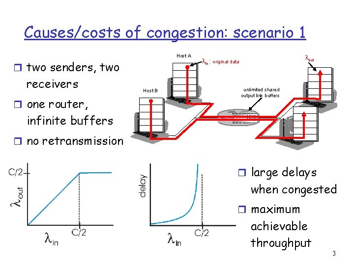
Causes/costs of congestion: scenario 1 Host A r two senders, two receivers r one router, Host B lout lin : original data unlimited shared output link buffers infinite buffers r no retransmission r large delays when congested r maximum achievable throughput 3

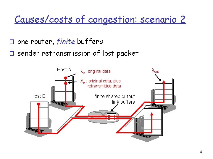
Causes/costs of congestion: scenario 2 r one router, finite buffers r sender retransmission of lost packet Host A lin : original data lout l'in : original data, plus retransmitted data Host B finite shared output link buffers 4

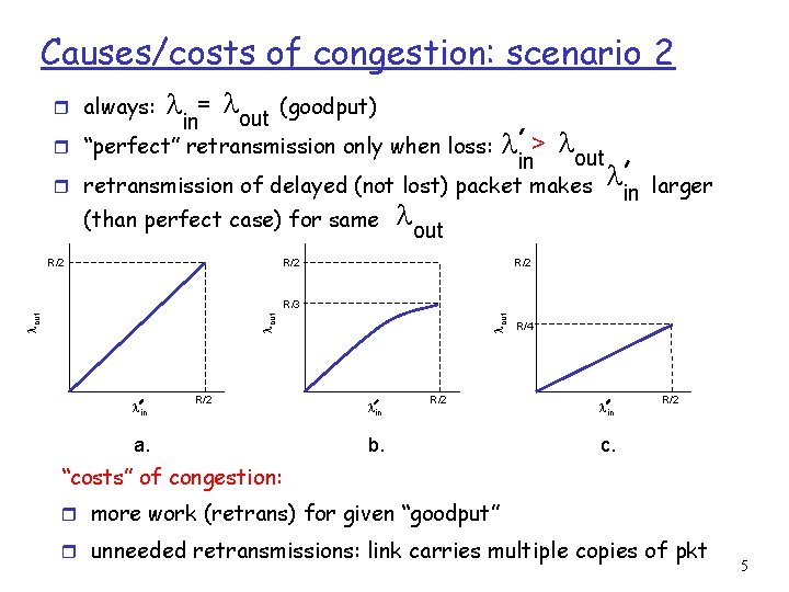
Causes/costs of congestion: scenario 2 = l (goodput) out in r “perfect” retransmission only when loss: r always: l l > lout in r retransmission of delayed (not lost) packet makes (than perfect case) for same R/2 l lout R/2 in larger R/2 lin R/2 a. lout R/3 lin R/2 b. R/4 lin R/2 c. “costs” of congestion: r more work (retrans) for given “goodput” r unneeded retransmissions: link carries multiple copies of pkt 5

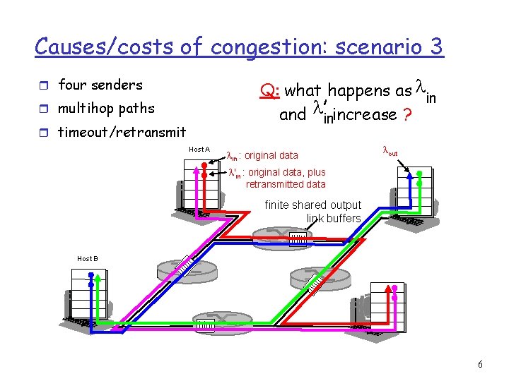
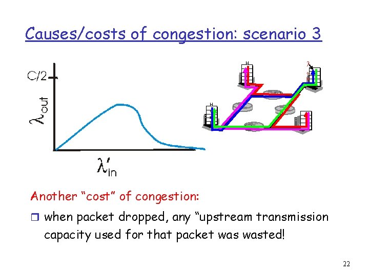
Causes/costs of congestion: scenario 3 Q: what happens as lin and linincrease ? r four senders r multihop paths r timeout/retransmit Host A lin : original data lout l'in : original data, plus retransmitted data finite shared output link buffers Host B 6

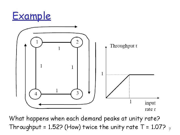
Example What happens when each demand peaks at unity rate? Throughput = 1. 52? (How) twice the unity rate T = 1. 07? 7

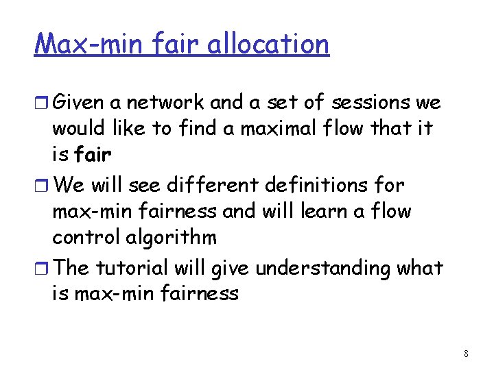
Max-min fair allocation r Given a network and a set of sessions we would like to find a maximal flow that it is fair r We will see different definitions for max-min fairness and will learn a flow control algorithm r The tutorial will give understanding what is max-min fairness 8

How define fairness? r Any session is entitled to as much network use as is any other. r Allocating the same share to all. 9

Max-Min Flow Control Rule r The rule is maximizing the network use allocated to the sessions with the minimum allocation r An alternative definition: is to maximize the allocation of each session i under constraint that an increase in i’s allocation doesn’t cause a decrease in some other session allocation with the same or smaller rate than i 10

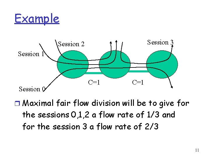
Example Session 3 Session 2 Session 1 Session 0 C=1 r Maximal fair flow division will be to give for the sessions 0, 1, 2 a flow rate of 1/3 and for the session 3 a flow rate of 2/3 11

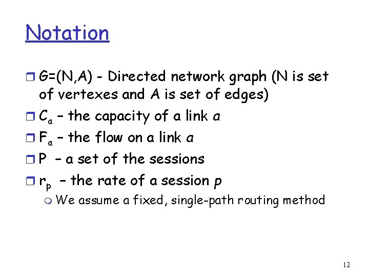
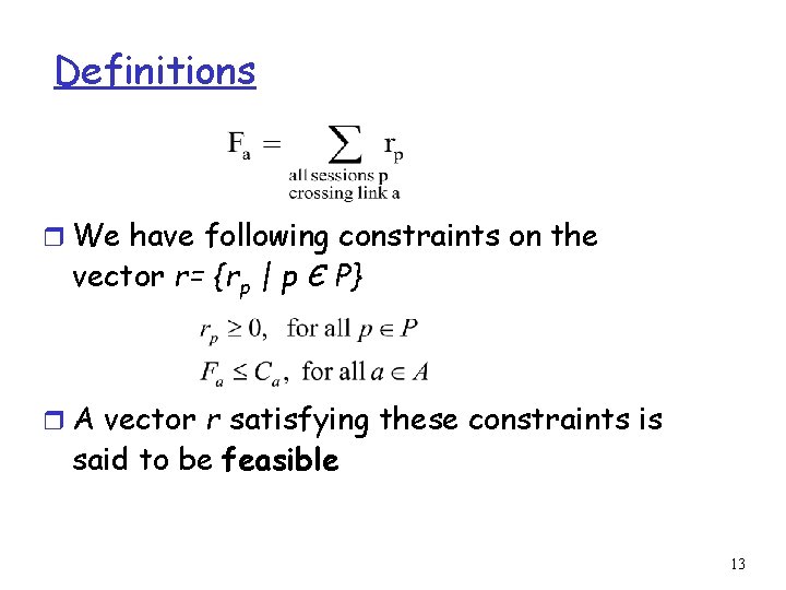
Notation r G=(N, A) - Directed network graph (N is set of vertexes and A is set of edges) r Ca – the capacity of a link a r Fa – the flow on a link a r P – a set of the sessions r rp – the rate of a session p m We assume a fixed, single-path routing method 12

Definitions r We have following constraints on the vector r= {rp | p Є P} r A vector r satisfying these constraints is said to be feasible 13

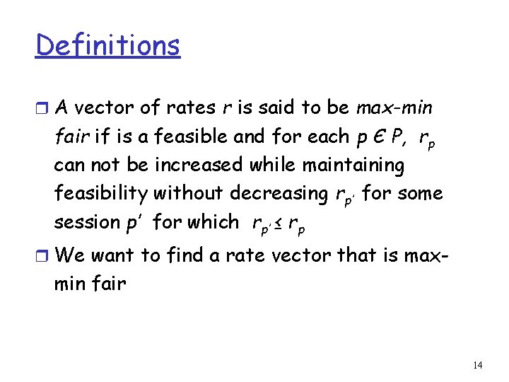
Definitions r A vector of rates r is said to be max-min fair if is a feasible and for each p Є P, rp can not be increased while maintaining feasibility without decreasing rp’ for some session p’ for which rp’ ≤ rp r We want to find a rate vector that is max- min fair 14

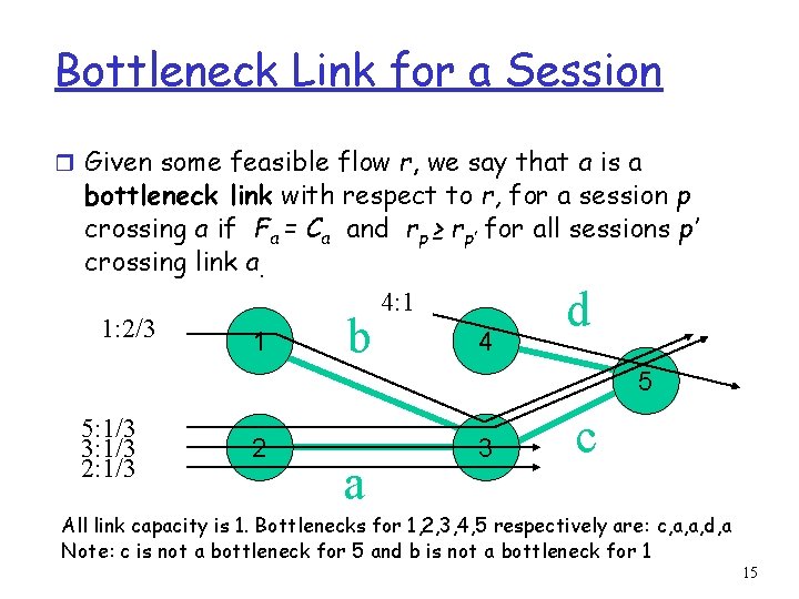
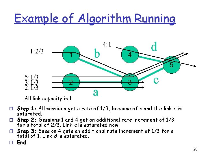
Bottleneck Link for a Session r Given some feasible flow r, we say that a is a bottleneck link with respect to r, for a session p crossing a if Fa = Ca and rp ≥ rp’ for all sessions p’ crossing link a. 4: 1 1: 2/3 1 4 5 d b 5: 1/3 3: 1/3 2 a 3 c All link capacity is 1. Bottlenecks for 1, 2, 3, 4, 5 respectively are: c, a, a, d, a Note: c is not a bottleneck for 5 and b is not a bottleneck for 1 15

Max-Min Fairness Definition Using Bottleneck r Theorem: A feasible rate vector r is max- min fair if and only if each session has a bottleneck link with respect to r 16

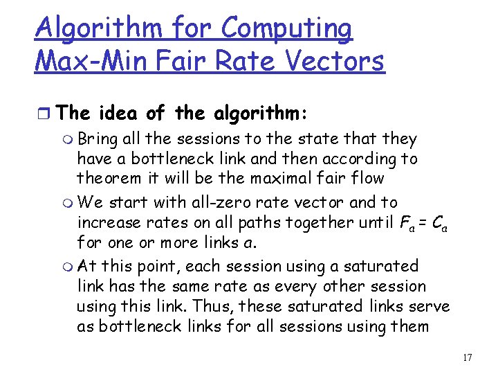
Algorithm for Computing Max-Min Fair Rate Vectors r The idea of the algorithm: m Bring all the sessions to the state that they have a bottleneck link and then according to theorem it will be the maximal fair flow m We start with all-zero rate vector and to increase rates on all paths together until Fa = Ca for one or more links a. m At this point, each session using a saturated link has the same rate as every other session using this link. Thus, these saturated links serve as bottleneck links for all sessions using them 17

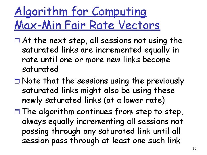
Algorithm for Computing Max-Min Fair Rate Vectors r At the next step, all sessions not using the saturated links are incremented equally in rate until one or more new links become saturated r Note that the sessions using the previously saturated links might also be using these newly saturated links (at a lower rate) r The algorithm continues from step to step, always equally incrementing all sessions not passing through any saturated link until all session pass through at least one such link 18

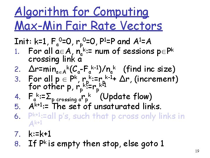
Algorithm for Computing Max-Min Fair Rate Vectors Init: k=1, Fa 0=0, rp 0=0, P 1=P and A 1=A 1. For all a A, nak: = num of sessions p Pk crossing link a 2. Δr=mina Ak(Ca-Fak-1)/nak (find inc size) 3. For all p Pk, rpk: =rpk-1+ Δr, (increment) for other p, rpk: =rpk-1 4. Fak: =Σp crossing arpk (Update flow) 5. Ak+1: = The set of unsaturated links. 6. Pk+1: =all p’s, such that p cross only links in Ak+1 7. k: =k+1 8. If Pk is empty then stop, else goto 1 19

Example of Algorithm Running 1: 2/3 1 b 4: 1 4 d 5 5: 1/3 3: 1/3 2 All link capacity is 1 a 3 c r Step 1: All sessions get a rate of 1/3, because of a and the link a is saturated. r Step 2: Sessions 1 and 4 get an additional rate increment of 1/3 for a total of 2/3. Link c is saturated now. r Step 3: Session 4 gets an additional rate increment of 1/3 for a total of 1. Link d is saturated. r End 20

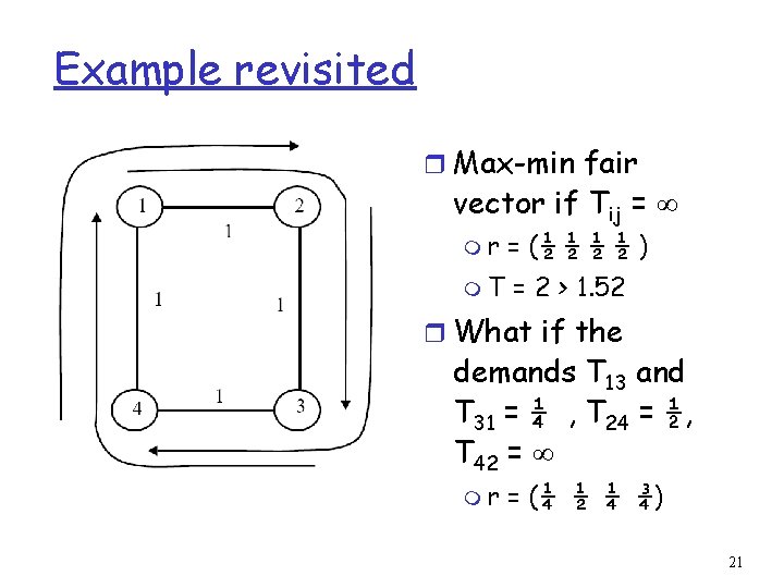
Example revisited r Max-min fair vector if Tij = ∞ mr = (½ ½ ) m. T = 2 > 1. 52 r What if the demands T 13 and T 31 = ¼ , T 24 = ½, T 42 = ∞ mr = (¼ ½ ¼ ¾) 21

Causes/costs of congestion: scenario 3 H o st A l o u t H o st B Another “cost” of congestion: r when packet dropped, any “upstream transmission capacity used for that packet wasted! 22

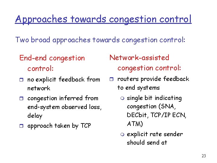
Approaches towards congestion control Two broad approaches towards congestion control: End-end congestion control: Network-assisted congestion control: r no explicit feedback from r routers provide feedback network r congestion inferred from to end systems m end-system observed loss, delay r approach taken by TCP m single bit indicating congestion (SNA, DECbit, TCP/IP ECN, ATM) explicit rate sender should send at 23

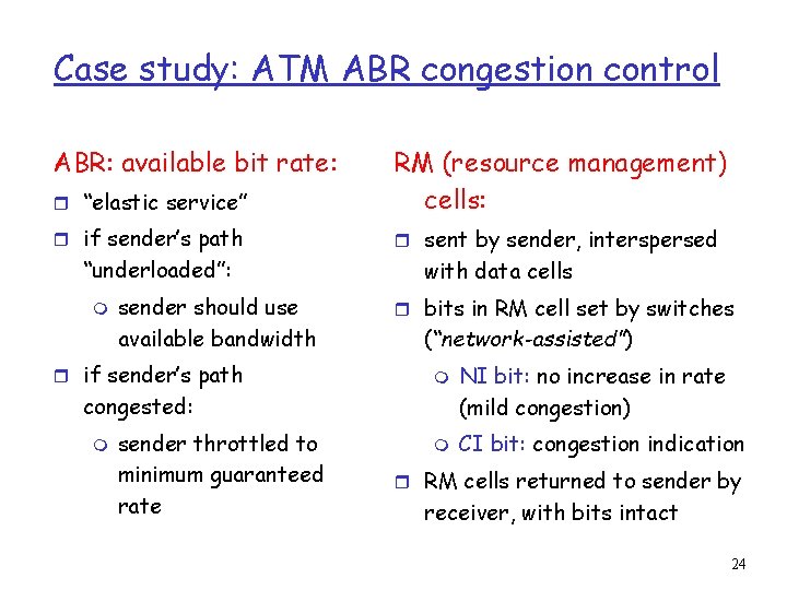
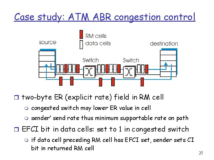
Case study: ATM ABR congestion control ABR: available bit rate: r “elastic service” RM (resource management) cells: r if sender’s path r sent by sender, interspersed “underloaded”: m sender should use available bandwidth r if sender’s path with data cells r bits in RM cell set by switches (“network-assisted”) m congested: m sender throttled to minimum guaranteed rate m NI bit: no increase in rate (mild congestion) CI bit: congestion indication r RM cells returned to sender by receiver, with bits intact 24

Case study: ATM ABR congestion control r two-byte ER (explicit rate) field in RM cell m congested switch may lower ER value in cell m sender’ send rate thus minimum supportable rate on path r EFCI bit in data cells: set to 1 in congested switch m if data cell preceding RM cell has EFCI set, sender sets CI bit in returned RM cell 25

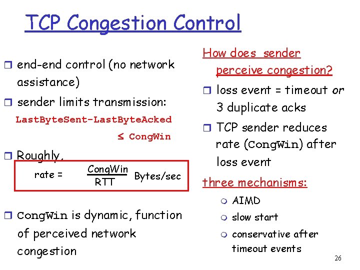
TCP Congestion Control r end-end control (no network assistance) r sender limits transmission: Last. Byte. Sent-Last. Byte. Acked Cong. Win r Roughly, rate = Cong. Win Bytes/sec RTT r Cong. Win is dynamic, function of perceived network congestion How does sender perceive congestion? r loss event = timeout or 3 duplicate acks r TCP sender reduces rate (Cong. Win) after loss event three mechanisms: m AIMD m slow start m conservative after timeout events 26

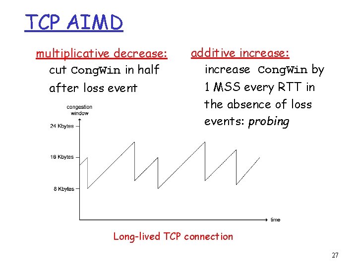
TCP AIMD multiplicative decrease: cut Cong. Win in half after loss event additive increase: increase Cong. Win by 1 MSS every RTT in the absence of loss events: probing Long-lived TCP connection 27

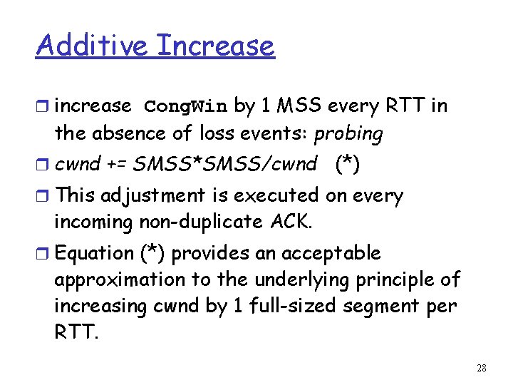
Additive Increase r increase Cong. Win by 1 MSS every RTT in the absence of loss events: probing r cwnd += SMSS*SMSS/cwnd (*) r This adjustment is executed on every incoming non-duplicate ACK. r Equation (*) provides an acceptable approximation to the underlying principle of increasing cwnd by 1 full-sized segment per RTT. 28

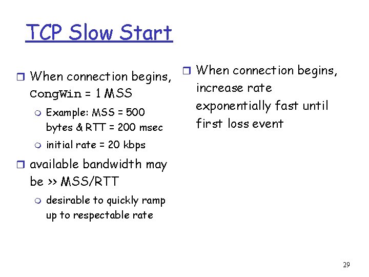
TCP Slow Start r When connection begins, Cong. Win = 1 MSS m m Example: MSS = 500 bytes & RTT = 200 msec r When connection begins, increase rate exponentially fast until first loss event initial rate = 20 kbps r available bandwidth may be >> MSS/RTT m desirable to quickly ramp up to respectable rate 29

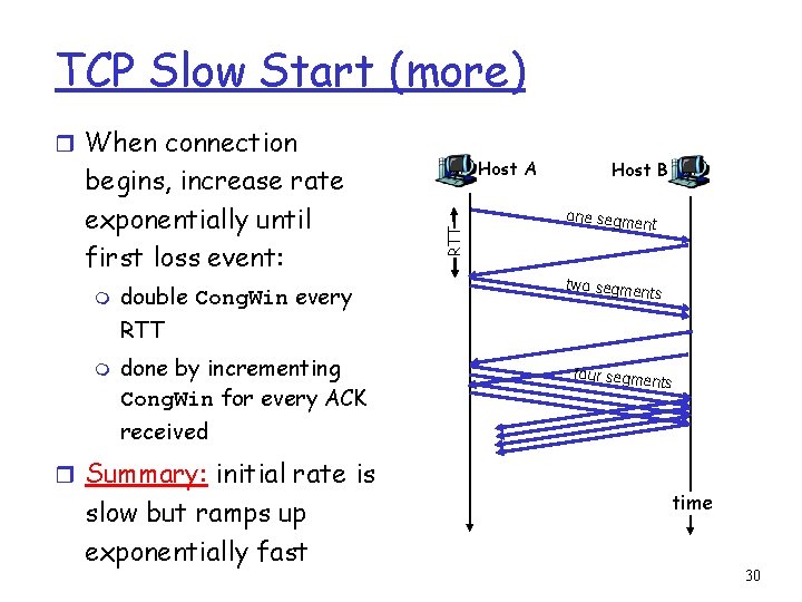
TCP Slow Start (more) r When connection m double Cong. Win every Host A RTT begins, increase rate exponentially until first loss event: Host B one segme nt two segme nts RTT m done by incrementing Cong. Win for every ACK four segme nts received r Summary: initial rate is slow but ramps up exponentially fast time 30

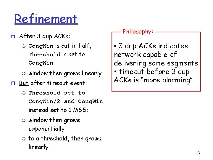
Refinement r After 3 dup ACKs: m m Cong. Win is cut in half, Threshold is set to Cong. Win window then grows linearly r But after timeout event: m Philosophy: • 3 dup ACKs indicates network capable of delivering some segments • timeout before 3 dup ACKs is “more alarming” Threshold set to Cong. Win/2 and Cong. Win instead set to 1 MSS; m m window then grows exponentially to a threshold, then grows linearly 31

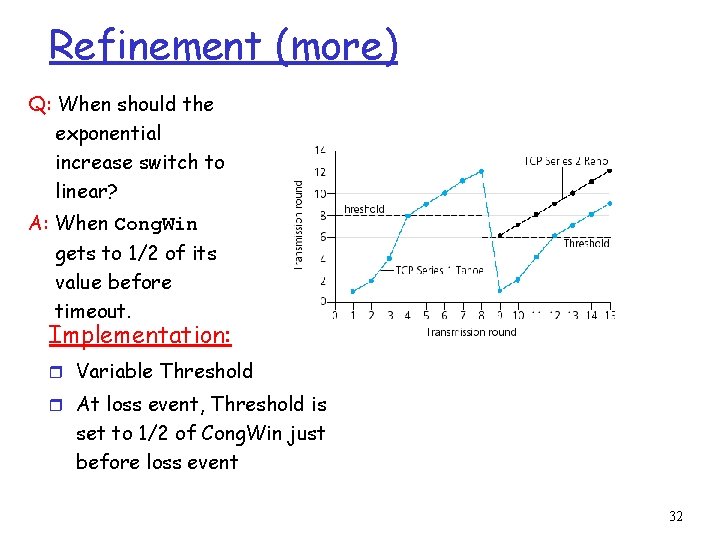
Refinement (more) Q: When should the exponential increase switch to linear? A: When Cong. Win gets to 1/2 of its value before timeout. Implementation: r Variable Threshold r At loss event, Threshold is set to 1/2 of Cong. Win just before loss event 32

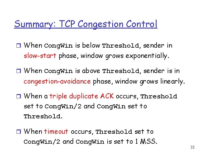
Summary: TCP Congestion Control r When Cong. Win is below Threshold, sender in slow-start phase, window grows exponentially. r When Cong. Win is above Threshold, sender is in congestion-avoidance phase, window grows linearly. r When a triple duplicate ACK occurs, Threshold set to Cong. Win/2 and Cong. Win set to Threshold. r When timeout occurs, Threshold set to Cong. Win/2 and Cong. Win is set to 1 MSS. 33

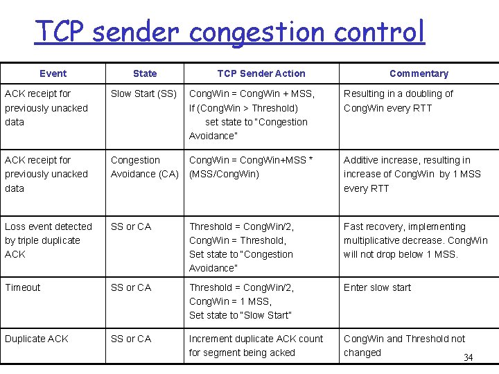
TCP sender congestion control Event State TCP Sender Action Commentary ACK receipt for previously unacked data Slow Start (SS) Cong. Win = Cong. Win + MSS, If (Cong. Win > Threshold) set state to “Congestion Avoidance” Resulting in a doubling of Cong. Win every RTT ACK receipt for previously unacked data Congestion Avoidance (CA) Cong. Win = Cong. Win+MSS * (MSS/Cong. Win) Additive increase, resulting in increase of Cong. Win by 1 MSS every RTT Loss event detected by triple duplicate ACK SS or CA Threshold = Cong. Win/2, Cong. Win = Threshold, Set state to “Congestion Avoidance” Fast recovery, implementing multiplicative decrease. Cong. Win will not drop below 1 MSS. Timeout SS or CA Threshold = Cong. Win/2, Cong. Win = 1 MSS, Set state to “Slow Start” Enter slow start Duplicate ACK SS or CA Increment duplicate ACK count for segment being acked Cong. Win and Threshold not changed 34

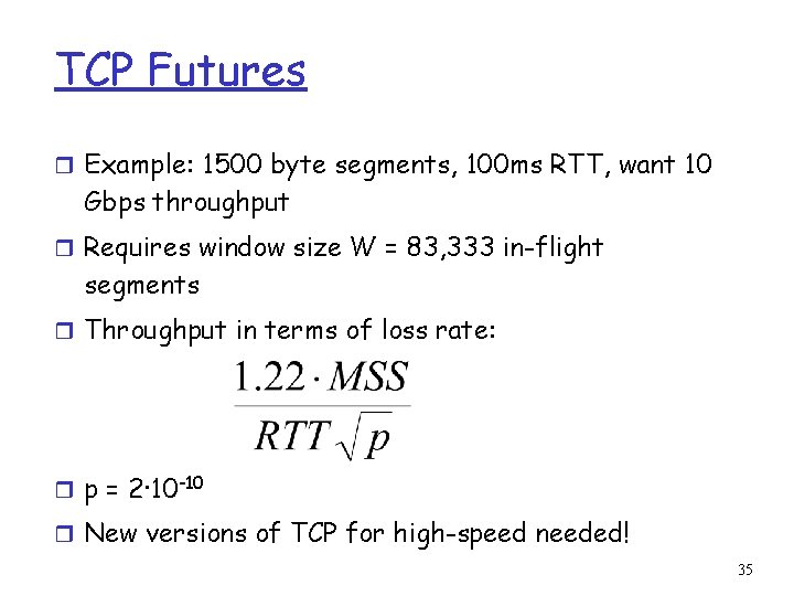
TCP Futures r Example: 1500 byte segments, 100 ms RTT, want 10 Gbps throughput r Requires window size W = 83, 333 in-flight segments r Throughput in terms of loss rate: r p = 2·10 -10 r New versions of TCP for high-speed needed! 35

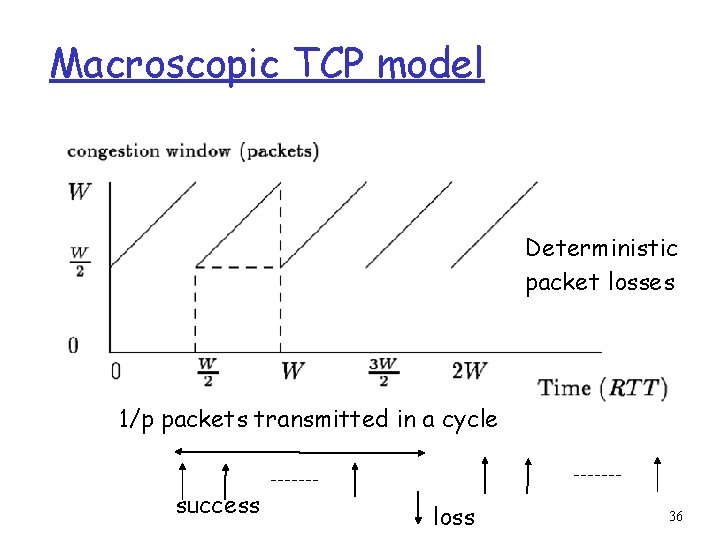
Macroscopic TCP model Deterministic packet losses 1/p packets transmitted in a cycle success loss 36

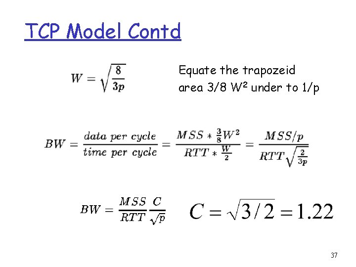
TCP Model Contd Equate the trapozeid area 3/8 W 2 under to 1/p 37

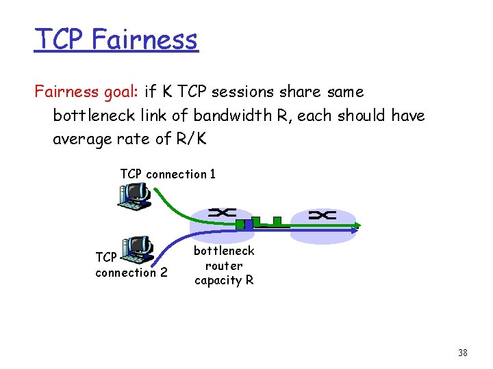
TCP Fairness goal: if K TCP sessions share same bottleneck link of bandwidth R, each should have average rate of R/K TCP connection 1 TCP connection 2 bottleneck router capacity R 38

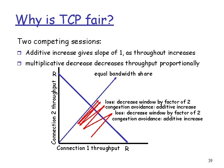
Why is TCP fair? Two competing sessions: r Additive increase gives slope of 1, as throughout increases r multiplicative decreases throughput proportionally equal bandwidth share Connection 2 throughput R loss: decrease window by factor of 2 congestion avoidance: additive increase Connection 1 throughput R 39

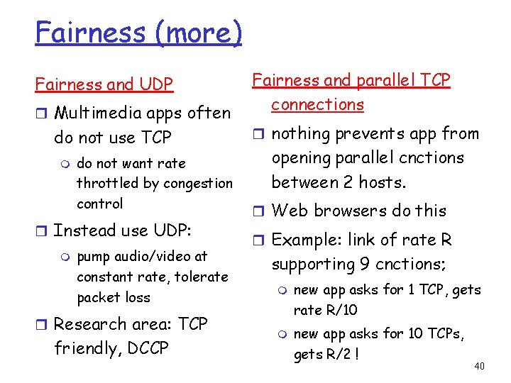
Fairness (more) Fairness and UDP r Multimedia apps often do not use TCP m do not want rate throttled by congestion control r Instead use UDP: m pump audio/video at constant rate, tolerate packet loss r Research area: TCP friendly, DCCP Fairness and parallel TCP connections r nothing prevents app from opening parallel cnctions between 2 hosts. r Web browsers do this r Example: link of rate R supporting 9 cnctions; m m new app asks for 1 TCP, gets rate R/10 new app asks for 10 TCPs, gets R/2 ! 40

Queuing Disciplines r Each router must implement some queuing discipline r Queuing allocates both bandwidth and buffer space: m Bandwidth: which packet to serve (transmit) next m Buffer space: which packet to drop next (when required) r Queuing also affects latency 41

Typical Internet Queuing r FIFO + drop-tail m Simplest m Used choice widely in the Internet r FIFO (first-in-first-out) m Implies single class of traffic r Drop-tail m Arriving packets get dropped when queue is full regardless of flow or importance r Important distinction: m FIFO: scheduling discipline m Drop-tail: drop policy 42

FIFO + Drop-tail Problems r Leaves responsibility of congestion control completely to the edges (e. g. , TCP) r Does not separate between different flows r No policing: send more packets get more service r Synchronization: end hosts react to same events 43

FIFO + Drop-tail Problems r Full queues m Routers are forced to have large queues to maintain high utilizations m TCP detects congestion from loss • Forces network to have long standing queues in steady -state r Lock-out problem m Drop-tail routers treat bursty traffic poorly m Traffic gets synchronized easily allows a few flows to monopolize the queue space 44

Active Queue Management r Design active router queue management to aid congestion control r Why? m Router has unified view of queuing behavior m Routers see actual queue occupancy (distinguish queue delay and propagation delay) m Routers can decide on transient congestion, based on workload 45

Design Objectives r Keep throughput high and delay low m High power (throughput/delay) r Accommodate bursts r Queue size should reflect ability to accept bursts rather than steady-state queuing r Improve TCP performance with minimal hardware changes 46

Lock-out Problem r Random drop m Packet arriving when queue is full causes some random packet to be dropped r Drop front m On full queue, drop packet at head of queue r Random drop and drop front solve the lock- out problem but not the full-queues problem 47

Full Queues Problem r Drop packets before queue becomes full (early drop) r Intuition: notify senders of incipient congestion m Example: early random drop (ERD): • If qlen > drop level, drop each new packet with fixed probability p • Does not control misbehaving users 48

Random Early Detection (RED) r Detect incipient congestion r Assume hosts respond to lost packets r Avoid window synchronization m Randomly mark packets r Avoid bias against bursty traffic 49

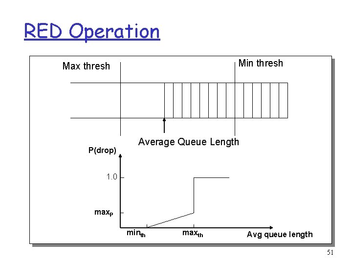
RED Algorithm r Maintain running average of queue length r If avg < minth do nothing m Low queuing, send packets through r If avg > maxth, drop packet m Protection from misbehaving sources r Else mark packet in a manner proportional to queue length m Notify sources of incipient congestion 50

RED Operation Min thresh Max thresh P(drop) Average Queue Length 1. 0 max. P minth maxth Avg queue length 51

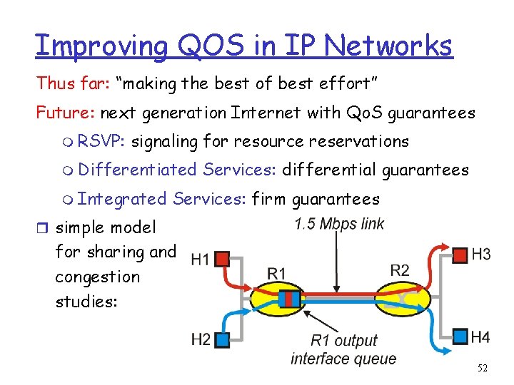
Improving QOS in IP Networks Thus far: “making the best of best effort” Future: next generation Internet with Qo. S guarantees m RSVP: signaling for resource reservations m Differentiated m Integrated Services: differential guarantees Services: firm guarantees r simple model for sharing and congestion studies: 52

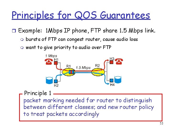
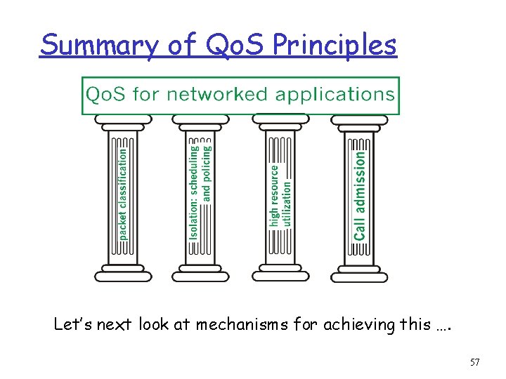
Principles for QOS Guarantees r Example: 1 Mbps IP phone, FTP share 1. 5 Mbps link. m bursts of FTP can congest router, cause audio loss m want to give priority to audio over FTP Principle 1 packet marking needed for router to distinguish between different classes; and new router policy to treat packets accordingly 53

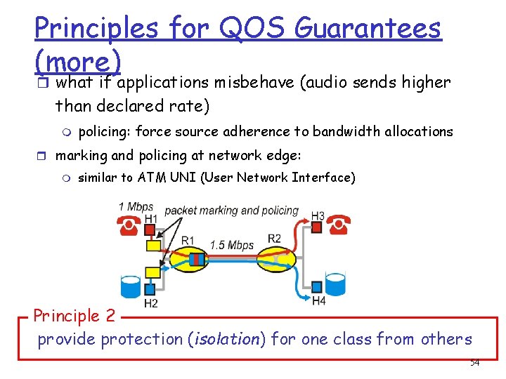
Principles for QOS Guarantees (more) r what if applications misbehave (audio sends higher than declared rate) m policing: force source adherence to bandwidth allocations r marking and policing at network edge: m similar to ATM UNI (User Network Interface) Principle 2 provide protection (isolation) for one class from others 54

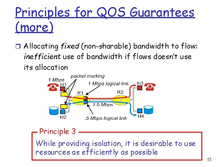
Principles for QOS Guarantees (more) r Allocating fixed (non-sharable) bandwidth to flow: inefficient use of bandwidth if flows doesn’t use its allocation Principle 3 While providing isolation, it is desirable to use resources as efficiently as possible 55

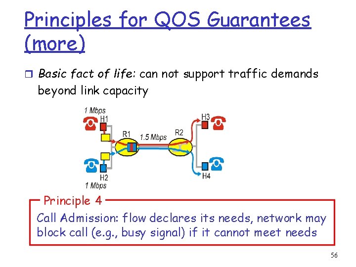
Principles for QOS Guarantees (more) r Basic fact of life: can not support traffic demands beyond link capacity Principle 4 Call Admission: flow declares its needs, network may block call (e. g. , busy signal) if it cannot meet needs 56

Summary of Qo. S Principles Let’s next look at mechanisms for achieving this …. 57

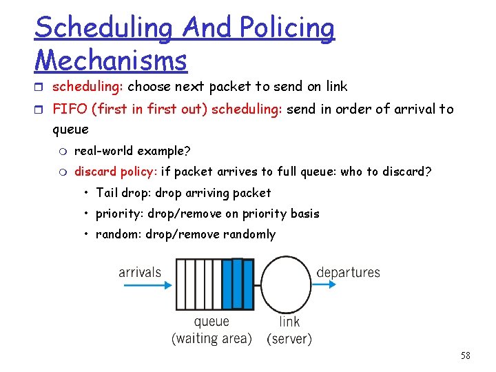
Scheduling And Policing Mechanisms r scheduling: choose next packet to send on link r FIFO (first in first out) scheduling: send in order of arrival to queue m real-world example? m discard policy: if packet arrives to full queue: who to discard? • Tail drop: drop arriving packet • priority: drop/remove on priority basis • random: drop/remove randomly 58

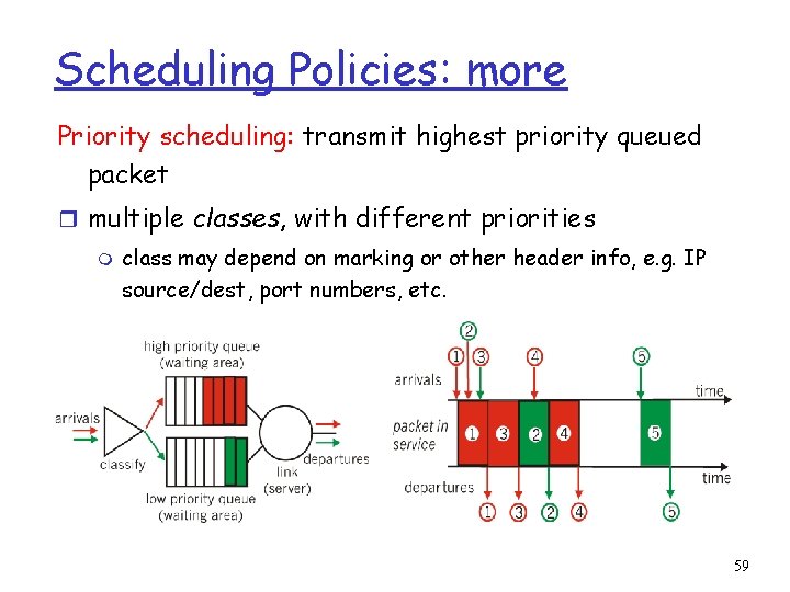
Scheduling Policies: more Priority scheduling: transmit highest priority queued packet r multiple classes, with different priorities m class may depend on marking or other header info, e. g. IP source/dest, port numbers, etc. 59

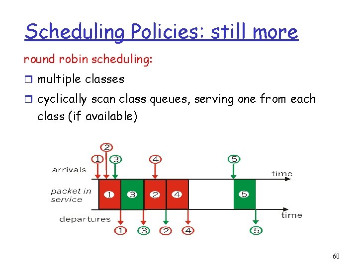
Scheduling Policies: still more round robin scheduling: r multiple classes r cyclically scan class queues, serving one from each class (if available) 60

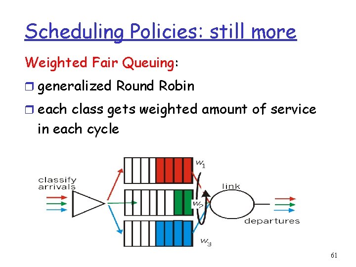
Scheduling Policies: still more Weighted Fair Queuing: r generalized Round Robin r each class gets weighted amount of service in each cycle 61

Deficit Weighted Round Robin (DWRR) r DWRR addresses the limitations of the WRR model by accurately supporting the weighted fair distribution of bandwidth when servicing queues that contain variable-length packets. r DWRR addresses the limitations of the WFQ model by defining a scheduling discipline that has lower computational complexity and that can be implemented in hardware. This allows DWRR to support the arbitration of output port bandwidth on high-speed interfaces in both the core and at the edges of the network. 62

DRR r In DWRR queuing, each queue is configured with a number of parameters: m m A weight that defines the percentage of the output port bandwidth allocated to the queue. A Deficit. Counter that specifies the total number of bytes that the queue is permitted to transmit each time that it is visited by the scheduler. The Deficit. Counter allows a queue that was not permitted to transmit in the previous round because the packet at the head of the queue was larger than the value of the Deficit. Counter to save transmission “credits” and use them during the next service round. 63

DWRR r In the classic DWRR algorithm, the scheduler visits each non-empty queue and determines the number of bytes in the packet at the head of the queue. r The variable Deficit. Counter isincremented by the value quantum. If the size of the packet at the head of the queue is greater than the variable Deficit. Counter, then the scheduler moves on to service the next queue. r If the size of the packet at the head of the queue is less than or equal to the variable Deficit. Counter, then the variable Deficit. Counter is reduced by the number of bytes in the packet and the packet is transmitted on the output port. 64

DWRR r A quantum of service that is proportional to the weight of the queue and is expressed in terms of bytes. The Deficit. Counter for a queue is incremented by the quantum each time that the queue is visited by the scheduler. r The scheduler continues to dequeue packets and decrement the variable Deficit. Counter by the size of the transmitted packet until either the size of the packet at the head of the queue is greater than the variable Deficit. Counter or the queue is empty. r If the queue is empty, the value of Deficit. Counter is set to zero. 65

DWRR Example Queue 1: 50% BW, quantum[1] =1000 300 400 600 Queue 2: 25% BW, quantum[2] =500 400 300 400 Queue 3: 25% BW, quantum[3] =500 400 300 600 Modified Deficit Round Robin gives priority to one say Vo. IP class 66

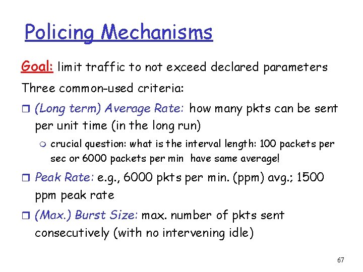
Policing Mechanisms Goal: limit traffic to not exceed declared parameters Three common-used criteria: r (Long term) Average Rate: how many pkts can be sent per unit time (in the long run) m crucial question: what is the interval length: 100 packets per sec or 6000 packets per min have same average! r Peak Rate: e. g. , 6000 pkts per min. (ppm) avg. ; 1500 ppm peak rate r (Max. ) Burst Size: max. number of pkts sent consecutively (with no intervening idle) 67

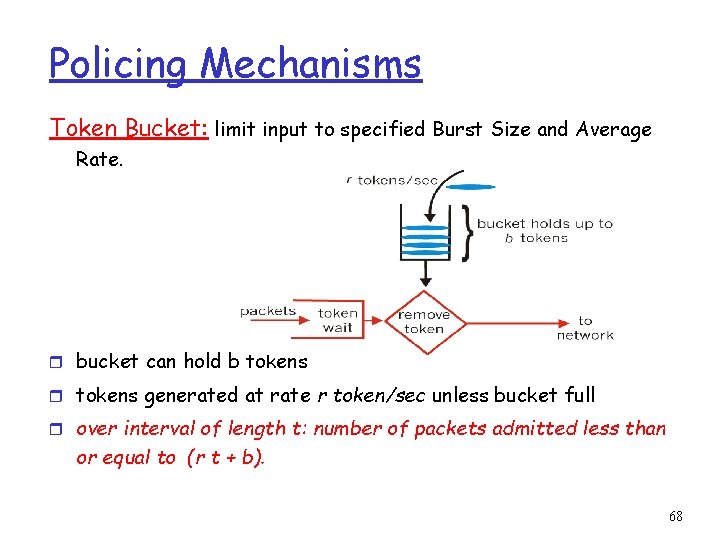
Policing Mechanisms Token Bucket: limit input to specified Burst Size and Average Rate. r bucket can hold b tokens r tokens generated at rate r token/sec unless bucket full r over interval of length t: number of packets admitted less than or equal to (r t + b). 68

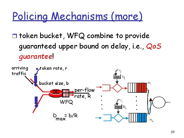
Policing Mechanisms (more) r token bucket, WFQ combine to provide guaranteed upper bound on delay, i. e. , Qo. S guarantee! arriving traffic token rate, r bucket size, b WFQ per-flow rate, R D = b/R max 69