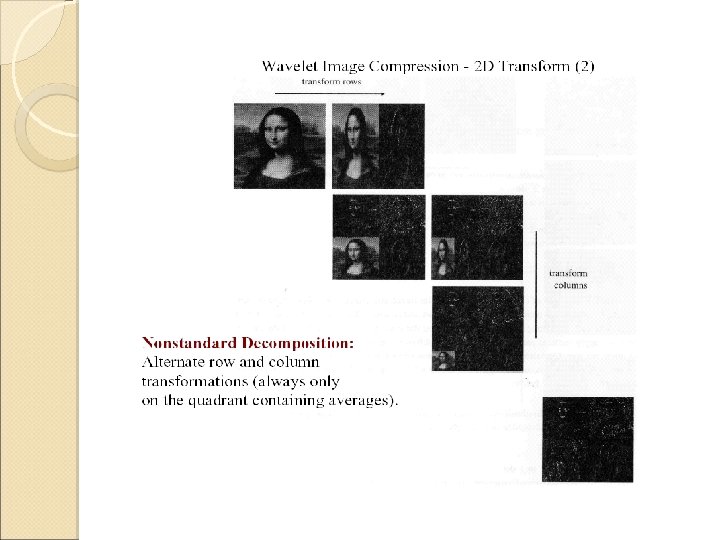
Wavelets Story begins with a functional linear subspace
 transforms")
Wavelets Story begins with a functional linear subspace spanned by Multi-Resolution Analysis (MRA) transforms to a hierarchy of subspaces, such that Analysis functions achieved by Wavelets

Why? Coverage of time-freq. space w Heisenberg box T time-freq. plane

Ahhhh Aeeee Spectral domain can be more informative

Why? w Heisenberg box T time-freq. plane

Problems? Ahhhh Aeeee But when?

Spatial-Spectral Localization Wavelets provide tradeoff

Spatial-Spectral Localization w Heisenberg Uncertainty Heisenberg box T time-freq. plane

Discrete Wavelet Transform w T
 Equation since ‘approx. ’ ‘detail’ spaces and")
How? Scaling (refinement) Equation since ‘approx. ’ ‘detail’ spaces and

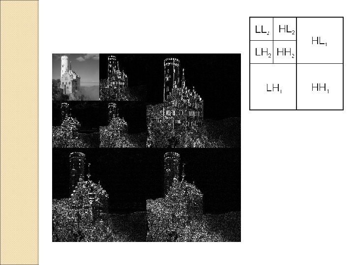
Sub-Spaces Cascade

Orthogonal Wavelets

Orthogonal Wavelets Inverse
![j ----- j y ----- y Trans. a 0 [1] a 1 [1] a](http://slidetodoc.com/presentation_image_h2/bd4ddd3121b72b6ab6279259bed4bf7e/image-13.jpg "j ----- j y ----- y Trans. a 0 [1] a 1 [1] a")
j ----- j y ----- y Trans. a 0 [1] a 1 [1] a 0 [2] a 1 [2] a 0 [3] a 1 [3] a 0 [4] = d 1 [4] a 0 [5] d 1 [5] a 0 [6] d 1 [6] Orthogonality j ----- j y ----- y Matrix Form a 1 [1] a 0 [1] a 1 [2] a 0 [2] a 1 [3] a 0 [3] d 1 [4] = a 0 [4] d 1 [5] a 0 [5] d 1 [6] a 0 [6] Bi-orthogonality ~ ---j ~ ---y ~ ---- y Inv. trans. a 1 [1] a 0 [1] a 1 [2] a 0 [2] a 1 [3] a 0 [3] d 1 [4] = a 0 [4] d 1 [5] a 0 [5] d 1 [6] a 0 [6]
 Design Basic requirements: • Admissibility (low-pass) (single constraint) • Orthogonality ( nonlinear")
Filter (Wavelet) Design Basic requirements: • Admissibility (low-pass) (single constraint) • Orthogonality ( nonlinear constraints) • Conditions on g • Given h, g is given by

Sparse Representation Smooth functions well approx. by Fourier ◦ High-frequency coefficients are roughly zero Piecewise smooth less ◦ All wavelengths respond to discontinuities Wavelets Design localization overcomes that Principles: ◦ Compact support ◦ Vanishes on smoothness (vanishing moments)

Vanishing Moments An analytic notion of smooth functions: polynomials The i. iii. iv. v. i. following are equivalent: The wavelet y has p vanishing moments The filter h has p vanishing moments and its p-1 derivatives are zero at w=0 and its p-1 derivatives are zero at w=p For any polynomials of degree k Smooth funcs. locally a polynomial (Taylor) low

Compact Support The scaling func. support is equal to the length of h. If h in [N 1, N 2] then y in [(N 1 -N 2+1)/2, (N 2 -N 1+1)/2] Sparsity at the cost of other attributes (less dofs) For example: Wavelets with p vanishing moments are at least 2 p-1
 Haar ◦ The only on of length 2, the anti-symmetric")
Example Wavelets (finite filters) Haar ◦ The only on of length 2, the anti-symmetric one Length 4: ◦ 3 conditions: ◦ 1 d parameterization: ◦ Daubechies-4 by a=p/3 with 2 V. M. (maximal) Length 6: …

Compression vs. JPEG image, file size 30081 bytes, Wavelets-based, file size compression ratio 19. 6. 30987 bytes, compression ratio 19. 0.

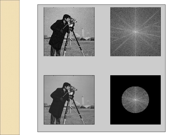
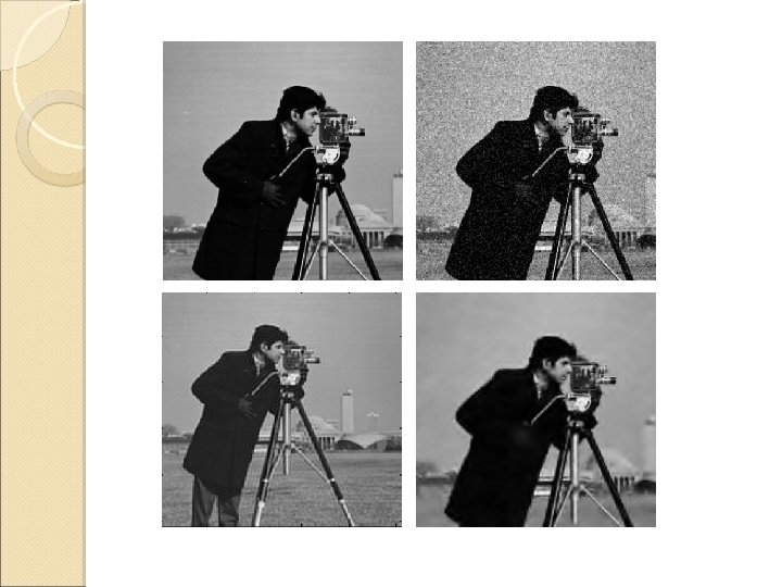
Noise Removal Random, spatially independent noise, is equally distributed over the spectrum But the piecewise smooth signal isn’t Solution: drop high-freq components (ringing), or threshold (and keep edges sharp / avoid ringing).
 usually minimize A ‘filters’ the right direction")
Preconditioning Iterative linear solvers for (A PSD) usually minimize A ‘filters’ the right direction e, how? A = Laplacian => The solution slowly solved on the low- freq. Preconditioning is about undoing this filtration Wavelets are localized in freq. and therefore match different levels of
![Interpolation Given N points, we can produce more by interpreting them as aj[n] and](http://slidetodoc.com/presentation_image_h2/bd4ddd3121b72b6ab6279259bed4bf7e/image-26.jpg "Interpolation Given N points, we can produce more by interpreting them as aj[n] and")
Interpolation Given N points, we can produce more by interpreting them as aj[n] and viewing them at a 0[n]. Inverse DWT with no data Linear in the number of output nodes. Example: ◦ Lifted splines bi-orth. wavelets

Biorthgonal Wavelets Orthogonal Wavelets are design limited due to too many constraints Can’t be finite & symmetric, relatively large Relax the construction by using of dual scaling func. and dual wavelet: Analysis: Synthesis:
 Use ‘arbitrary’ matrix and its inverse…")
Biorthgonal Wavelets Rather than: where W* =W-1 (orthogonality) Use ‘arbitrary’ matrix and its inverse… (constructed by dilations and translations of course. . )

Biorthgonal Wavelets The dual story: ◦ Scaling eqns ◦ Admissibility ◦ Birothogonality conds: “linear constaints”

Design Compact Support ◦ if and then Vanishing Moments ◦ The number of vanishing moments w= p equals the number of zeros of at Symmetry ◦ It is possible to construct finite symmetric and antisymmetric Odd lengths are also possible The filters and dual filters can be exchanged
 same parity")
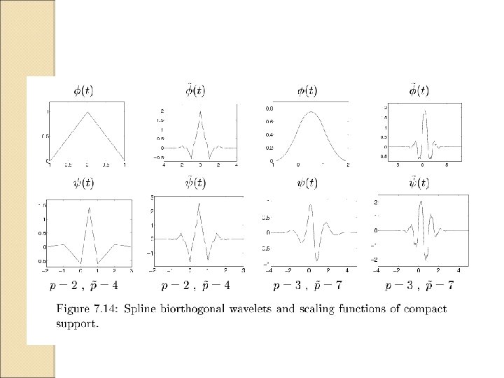
Example B-Wavelets Splines is the number of V. M. (free param. ) same parity as. The minimum length dual filter is given by

The Spectral Picture As we know is 2 p-periodic For real wavelets, And we know: Power Spectrum
 steps can be identified: ◦")
Lifting scheme Let’s review the Haar WT Three (non-normalized) steps can be identified: ◦ Split: reordering into even + odd ◦ Predict: pred. odd based on even and storing the difference. ◦ Update: (just) make sure that

Lifting scheme Inverse is just: ◦ Undo update: ◦ Undo predict: ◦ Merge: Properties: ◦ In-place ◦ No Fourier Analysis! (boundary conditions, non-regular domains, other spatial dependencies)
 obtained using polynomial prediction. Linear case: Zero on")
Example: Splines and the (subdivision methods) obtained using polynomial prediction. Linear case: Zero on linear functions Gives the biorthogonal (2, 2) of Cohen-Daubechies. Feauveau Linear time + avoids fitting polynomials.

Second Generation Wavelets Vary in space – no Fourier analysis ◦ Interval boundary conditions ◦ Irregular samples ◦ Weighted measure Still maintain ◦ Stable basis (orthogonal / biorthogonal) ◦ Locality in space / time & frequency ◦ MRA, cascade construction

Second Generation Wavelets Concept of V. M. regularity remains

Operator Notation Convolution matrices in case of 1 st Generation Wavelets

Lifting Scheme Sj parameterizes the lifted wavelets Use Sj to locally “design” the wavelets ◦ Begin with simple wavelets, e. g. , the Lazy wavelets
![Unbalanced Haar a[n] no longer at points, but on intervals a[n] Constants give zero](http://slidetodoc.com/presentation_image_h2/bd4ddd3121b72b6ab6279259bed4bf7e/image-41.jpg "Unbalanced Haar a[n] no longer at points, but on intervals a[n] Constants give zero")
Unbalanced Haar a[n] no longer at points, but on intervals a[n] Constants give zero detail
- Slides: 41