Wavelet Transform A Presentation By Subash Chandra Nayak

Wavelet Transform A Presentation By Subash Chandra Nayak 01 EC 3010 IIT Kharagpur INDIA

Introduction to the world of transform • What are transforms : • • • A mathematical operation that takes a function or sequence and maps into another one General Form : - Examples : Laplace, Fourier, DTFT, DFT, FFT, z-transform

Fourier Transform Mathematical Form : - Notes : Fourier transform identifies all spectral components present in the signal, however it does not provide any information regarding the temporal (time) localization of the components

Fourier Transform : : Limitations • Signals are of two types # Stationary # Non – Stationary • Non stationary signals are those who have got time varying spectral components. . . FT gives only provides the existence of the spectral components of the signal. . . But does not provide any information on the time occurrence of spectral components • Explanation The basis function e-jwt stretches to infinity , Hence only analyzes the signal globally In order to obtain time-localization of spectral components , the signal need to be analyzed locally

Time – Frequency Representation • Instantaneous frequency : - • Group delay : - • Disadvantages of above expressions These equations though have a huge theoretical significance but are not easy to implement easily

Short-time Fourier Transform • • Also known as a STFT given as • w(t) : - windowing function generally a Gaussian pulse is used, other choices are rectangular , elliptic etc. . Maps 1 D function to 2 D time-frequency domain • • Advantages : # Gives us time-frequency description of the signal # Overcomes the difficulties of Fourier transform by use of windowing functions

STFT : : Disadvantages • Heisenberg Principle : One can not get infinite time and frequency resolution beyond Heisenberg’s Limit • Trade offs : • • Wider window Good frequency resolution , Poor time resolution Narrower window Good time resolution , Poor frequency resolution

Wavelet Transform • • Overcomes the shortcoming of STFT by using variable length windows : : i. e. Narrower window for high frequency thereby giving better time resolution and Wider window at low frequency thereby giving better frequency resolution Heisenberg’s Principle still holds • Mathematical form: - where x(t) = given signal tau = translation parameter s = scaling parameter = 1/f phi(t) = Mother wavelet , All kernels are obtained by scaling and/or translating mother wavelet

Continuous Wavelet transform • The kernel functions used in wavelet transform are all obtained from one prototype function known as mother wavelet , by scaling and/or translating it • Here a = scale parameter b = translation parameter • Continuous Wavelet transform

CWT (Contd. . ) • In order to become a wavelet a function must satisfy the above two conditions

Inverse wavelet transform

Examples of wavelets

Constant Q-filtering • CWT can be rewritten as • A special property of the above filter defined by the mother wavelet is that they are Constant-Q filters • Q factor = Center frequency/Bandwidth • Hence the filter defined by wavelet increases their Bandwidth as scale increases ( i. e. center frequency increases ) • This boils down to filter bank implementation of discrete wavelet transform

Filter Banks : : General Structure • Condition for Perfect Reconstruction

Filter bank (Contd. . ) • Product filter Now let’s define product filter as : P 0(z) = F 0(z)H 0(z) And Normalized Product filter as P(z) = z. L P 0(z) where L = delay in total process So the PR condition boils down to this realationship P(z) – P(-z) = 2

Harr Filter Bank Note that f 0(n) and f 1(n) are non-causal. . . Hence here Unit delay is required to implement it hence here L=1

Product filter P(w) is said to be halfband filter because of its symmetry Also P(w) + P(w + pi) = 2

Product filter II • P(w) should be as flat as possible around 0 and pi. The more is the flatness of P(w) around 0 and pi the better the Product filter is. Hence P(w) is always tried to be designed as a MAXFLAT Filter • Order of filter : : p p = (L+1)/2 ; L = number of delay elements • Methods of determination of P(z) # Duabechies method # Meyer methods • Both of the above methods give us P(z) for a given order “p”. The higher is the order the better is the filter but at the same time it will require more hardware complexity

Spectral factorization • • • The spectral factorization is the problem of finding h 0(z) once P(z) is known Linear Phase Factorization H 0(z) and F 0(z) are of different degree. Gives filter with linear phase Orthogonal Factorization H 0(z) and F 0(z) are of same degree. Gives filter with nonlinear phase. Daubechies family of filters belongs to this category. For orthogonal filter

Discrete wavelet Transform • • Discrete domain counterpart of CWT Implemented using Filter banks satisfying PR condition Represents the given signal by discrete coefficients {dk, n} DWT is given by

Scaling Function • • These are functions used to approximate the signal up to a particular level of detail For Harr System Harr Scaling Function

Refinement equation and wavelet Equation • Refinement equation is an equation relating to scaling function and filter coefficients Refinement Equation • Wavelet equation is an equation relating to wavelet function and filter coefficients • By solving the above two we can obtain the scaling and wavelet function for a given filter bank structure Wavelet Equation

DWT Implementation a(k, n) g`[n] d(k+1, n) 2 a(k+1, n) h`[n] 2 Decomposition g`[n] 2 h`[n] 2 d(k+2, n) a(k+2, n) 2 g[n] 2 h[n] + 2 g[n] 2 h[n] a(k+1, n) Reconstruction We have only shown the above implementation for the Haar Wavelet, however, as we will see later, this implementation – subband coding – is applicable in general. +

DWT Sub-band Decomposition x[n] g[n] Length: 256 B: /2 ~ Hz h[n] 2 w |G(jw)| g[n] h[n] 2 d 2: Level 2 DWT Coeff. Length: 64 B: /8 ~ /4 Hz /2 - /2 Length: 256 B: 0 ~ /2 Hz 2 d 1: Level 1 DWT Coeff. Length: 128 B: /4 ~ /2 Hz |H(jw)| Length: 512 B: 0 ~ 2 g[n] 2 d 3: Level 3 DWT Coeff. Length: 128 B: 0 ~ /4 Hz - h[n] 2 Length: 64 B: 0 ~ /8 Hz ……. - /2 w

Sub-band coding

Some Important properties of wavelets • Compact Support : • Finite duration wavelets are called compactly supported in time domain but are not band-limited in frequency. Can be implemented using FIR filters • Examples Harr, Daubechies, Symlets , Coiflets • Narrow band wavelets are called compactly supported in frequency domain. Can be implemented using IIR filters • Examples Meyer’s wavelet

Some Important properties of wavelets • • Symmetry Symmetric / Antisymetric wavelets have got liner-phase Orthogonal wavelets are asymmetric and have a non-linear phase Biorthogonal wavelets are asymmetric but have got linear phase can be implemented using FIR filters • • Vanishing Moment pth vanishing moment is defined as • The more the number of moments of a wavelets are zero the more is its compressive power

Some Important properties of wavelets • Smoothness • is roughly the number of times a function can be differentiated at any given point • Closely related to vanishing Moments • Smoothness provides better numerical stability • It also provides better reconstruction propertiy

2 D DWT • Generalization of concept to 2 D • 2 D functions images f(x, y) I[m, n] intensity function • Why would we want to take 2 D-DWT of an image anyway? – Compression – Denoising – Feature extraction • Mathematical form

Implementation of 2 D-DWT COLUMNS ROWS …… ROWS COLUMNS …… ~ H 2 1 INPUT IMAGE COLUMNS ROWS ~ G 2 1 COLUMNS INPUT IMAGE LL LH HL HH ~ H 1 2 LL ~ G 1 2 LH ~ H 1 2 HL ~ G 1 2 HH LLL LLH LHL LHH HL LH HH LLH LHL LHH LL HL LH HH

Up and Down … Up and Down 2 1 Downsample columns along the rows: For each row, keep the even indexed columns, discard the odd indexed columns 1 2 Downsample columns along the rows: For each column, keep the even indexed rows, discard the odd indexed rows 2 1 Upsample columns along the rows: For each row, insert zeros at between every other sample (column) 1 2 Upsample rows along the columns: For each column, insert zeros at between every other sample (row)

Reconstruction LL LH HL 1 2 H 2 1 1 2 G 1 2 H ORIGINAL IMAGE 2 1 HH 1 2 G H G

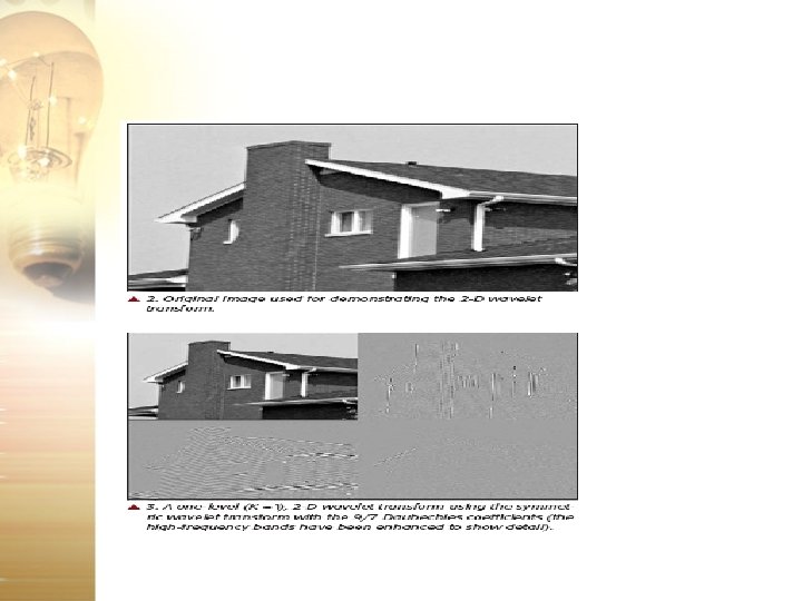
DWT in Work

DWT at work

DWT at work

Applications of wavelets • There a lots of uses of wavelets. . The most prominent application of wavelets are • • • Computer and Human Vision FBI Finger Print compression Image compression Denoising Noisy data Detecting self-similar behavior in noisy data Musical Notes synthesis Animations • •

Things that I didn’t Cover • Different algorithms for getting Product filter, max-flat filter realization, spectral factorization , solutions for refinement and wavelet equations and many more • Noble Identity, modulation matrix, Polyphase matrix forms • MRA , Mallat’s pyramidal algorithm • Lifting • Basic Vector algebra needed for wavelet analysis ( It’s too mathematical to present ) • Orthogonality, biorthogonality, frames • Vector algebra approach for wavelets • Wavelet for denoising and many more. . . .