Water Supply Engineering Water Supply and Sanitation in

Water Supply Engineering • Water Supply and Sanitation in India – Poor, Inadequate , Low by International Standards • Local Government Institutions – Weak in Operation and Maintenance, Lack resources to carry out functions • Access to improved water sources – 72% (1990) and 88% (2008) • Urban - 96%; Rural - 84%; Total - 88%

• Average Urban Water Use – 150 L/Capita/day • Annual Investment in Water Supply and Sanitation – US$5/capita • Indian Norms – Improved water supply exists if at least 40 L/capita/day of safe drinking water are provided within distance of 1. 6 km or 100 m elevation difference (to be relaxed as per field conditions). One pump per 250 persons

• 35 cities > 1 million population distribute water for few hours • According to Asian Development Bank (ADB) study in 2007 – average duration of water supply in 20 cities was 4. 3 hours/day. • Longest duration of supply – 12 hrs/day in Chandigarh and lowest duration of supply - 0. 3 hrs/day in Rajkot • According to World Bank – performance indicators not comparable with average International Standards • No city had continuous supply

• Depleting Groundwater Table and deteriorating Groundwater quality threaten both urban and rural water supply in india • Surface water – Pollution, scarcity, Conflicts among users (Eg. , conflict over Cauvery water among Tamil Nadu and Karnataka) • Bangalore – Cauvery water pumped since 1974. Cauvery Stage IV (Phase II) project includes supply of 500, 000 cubic meter of water per day over a distance of 100 km

• Water supply and Sanitation – State Responsibility under Indian constitution • States may give responsibility to Panchayati Raj Institutions (PRI) in rural areas or municipalities in urban areas, called Urban Local Bodies (ULB) • At present, states generally plan, design and execute (often operate) through state departments (Public Health Engineering or Rural Development Engineering) or state water boards • Highly centralized decision making approvals at state affect management of water supply and sanitation services • Planning Commission Report 2003 – trend to decentralize capital investment to engineering departments at district level and operation and maintenance to district and gram panchayat levels

Central Ministries Ministry of Rural Development - Rural Water Supply Ministry of Housing and Urban Poverty Alleviation – Urban Water Supply Department of Drinking Water Supply Only advisory capacity and limited role in funding

• Typically, a state-level agency is in charge of planning and investment, while local government (ULBs) is in charge of operation and maintenance • Private Sector Participation – limited role on behalf of ULBs. – Jamshedpur Utilities and Services Company (JUSCo) – Lease contract for Jharkhand, Management contract in Haldia(West bengal), Mysore (Karnataka) and Contract for reduction of non-revenue water in Bhopal (MP) – Veolia (French Water Company) – management contract in 3 cities (Hubli, Belgaum and Gulbarga) in Karnataka in 2005 – Thames Water – Hydrocomp – contract for Latur city (Maharastra) – SPML - Bulk water supply project for Bhiwandi (Maharastra) on Build-Operate-Transfer (BOT) basis

Innovative Approaches • Demand-Driven Approach – Swajaldhara – community participation • Public-Private Partnerships (PPP) to improve continuity of water supply in karnataka • Micro-credit to women in order to improve access to water

Investment and Financing • Increased during Ist decade of 21 st century • Central Government grants under Jawaharlal Nehru National Urban Renewal Mission (JNNURM) and loans from Housing and Urban Development Corporation (HUDCO) • 11 th Five Year Plan (2007 – 2012) investments of Rs. 127025 crore for urban water supply and sanitation including urban storm water drainage and solid waste management – 55% central govt. , 28% state govt. , 8% Institutional financing ‘HUDCO’, 8% external agencies and 15% private sector

External Cooperation • Japan US$635 million – largest donor – Projects approved between 2006 and 2009 include Guwahati Water Supply Project (Phase I and II) in Assam – Kerala Water Supply Project (Phase II and III) – Hogenakkal Water Supply and Fluorosis Mitigation Project (Phase I and II) in Tamil Nadu – Goa Water Supply and Sewerage Project – Agra Water Supply Project – Amritsar Sewerage Project in Punjab – Orissa Integrated Sanitation Improvement Project – Bangalore Water Supply and Sewerage Project (Phase. II) • World bank US$130 million – financial support in Andhra Pradesh, Karnataka, Tamil Nadu, Uttaranchal and Punjab • Asian Development Bank • Germany

Planning Guidelines for Water Supply and Sewerage

Purpose • Identify service needs in the short, medium and long term in order to deliver defined service standards, social, environmental and financial outcomes • Evaluate options for delivering the defined outcomes • Determine the optimal strategy that delivers the defined outcomes at the lowest financial, social and environmental cost • Communicate the outcomes of the planning process to decision makers through a planning report

Key Principles • Include comprehensive and rigorous identification of all options to meet service levels • Iterative process which attempts to balance service needs with infrastructure, operation and maintenance, financial and environmental options • Key stakeholders identified and involved in planning stage

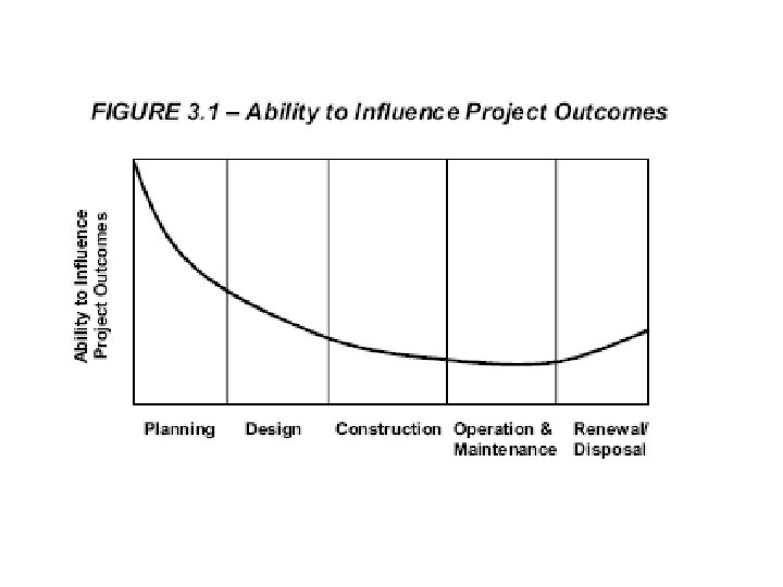
Why Planning is Important? • Planning stage – early stage of an initiative which influences the project outcomes, minimize risk and reduce costs • Investment in planning results in substantial dividends • Cost of planning is low (as compared to capital expenditure involved in construction and Operation and Maintenance)

Outcomes from effective planning include: • Common understanding of the issues, options and outcomes by all stakeholders • Cost effective Infrastructure investment program • Achievement of an optimal, financial, social and environmental result • Lower costs to the customer • Continued achievement of service standards • Protection of the natural and built environment • Minimization of risk • Appropriate solutions for available skill level

Issues stimulated for planning • • Changes in unit demands for services Variation in growth projections Adverse trends in customer service levels Changes in community attitudes Changes in technology Changes in regulatory requirements or guidelines Timeframes for the provision of critical infrastructure to meet service demands

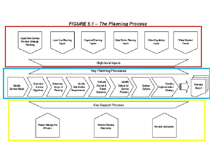
Higher Level Inputs High Level Input Typical Source of Information Service Provider Strategic Planning Information provides strategic direction for the delivery of water and sewerage services and storm water management. It would address matters such as customer service standards and financial, social and environmental objectives. Information would typically be provided from Ø Corporate plan Ø Business plan Ø Operations plan Ø Total Strategic Management Plan Ø Customer Service Standards Ø Environmental Management Plan - Iterative process. Land Use Planning Ø Strategic Land Use Plan Ø Priority Infrastructure Plan Ø Integrated Catchment Management Plan

Regional Planning Ø Regional and Sub Regional Planning Strategy Plans and Studies Ø Regional and Sub Regional Infrastructure Planning Studies State Water Planning Ø Water Resource Plan (WRP) Ø Resource Operations Plan Ø Resources Operations Licence (ROL) Ø Regional Water Supply Strategies Other Regulatory Inputs Ø Water Act Ø Environmental Protection Act Water Related Trends Issues covered : Ø Climate Change Ø Status of the Environment and Future Scenarios Ø Planning Trends (e. g. Integrated Water Management) Ø Trends in Technology ØRegulatory Trends Ø Trends in community perception ØTrends in customer needs

Key Elements • • • Identify Service Need Determine Service Objectives Determine Scope of Planning Identify Stakeholder Requirements Evaluate Current and Future Demands Identify Options for Service Provision Undertake Options Analysis Develop Implementation Strategy Outputs from the planning process

Key Support Processes • Project Management • Planning Information • Planning Resources

Terms • Design Period – It is the number of years for which the system or component is to be adequate • Design Population – The number of persons to be served • Design area – area to be served by the system or component for the residential, commercial and industrial districts and public areas • Design Flows – rates of consumption for the residential, commercial, industrial districts and public areas of the city

Design Periods for Project Components Sl. No. Component Design Period (Years) 1. Storage by Dams 50 2. Infiltration Works 30 3. Pump Sets (i)All Prime Movers except electric motors (ii) Electric Motors and Pumps 30 15 4. Water Treatment Units 15 5. Pipe connections to the several treatment units and other small appurtenances 30 6. Raw water and clear water conveying mains 30 7. Clear water reservoirs at the head works, balancing tanks and service reservoirs (over head or ground level) 15 8. Distribution system 30

Water Consumption for Various Purposes Sl. No Types of Consumption Normal Range (litres/capita/day) Average % 1. Domestic Consumption 65 -300 160 35 2. Industrial and Commercial Demand 45 -450 135 30 3. Public Uses including Fire Demand 20 -90 45 10 4. Losses and Waste 45 -150 62 25

Water Requirements for Domestic Use Sl. No. Description Amount of water in litres per head per day 1. Bathing 55 2. Washing of clothes 20 3. Flushing of Water Closet 30 4. Washing the house 10 5. Washing of Utensils 10 6. Cooking 5 7. Drinking 5 Total 135 litres

Water for Institutional Needs Sl. No. Institution Water Requirement (litres per head per day) 1. Hospitals (including Laundry) (a)No. of beds > 100 (b)No. of beds < 100 450 (per bed) 340 (per bed) 2. Hotels 180 (per bed) 3. Hostels 135 4. Boarding Schools/Colleges 135 5. Restaurants 70 (per seat) 6. Airports and Sea Ports 70 7. Day Schools/Colleges 45 8. Offices 45 9. Cinemas, Concert Halls and Theatres 15

Industrial Need Sl. No. Industry Unit of Production 1. Automobile Vehicle Water Requirements in Kilolitres per unit 40 2. Fertilizer Tonne 80 -200 3. Leather 100 kg(tonne) 4 4. Paper Tonne 200 -400 5. Steel Tonne 200 -250 6. Sugar 1 -2 7. Textile Tonne(cane crushed) 100 kg (goods) 8 - 14

Fire Fighting Demand • Empirical Formulae Sl. No. Authority Formulae (P in thousand) 1. Kuchling’s Formula Q (Litres/min. ) = 3182√P 31820 2. Freeman’s Formula Q (Litres/min. ) = 1136 34080 3. National Board of Underwriters Formula 41760 4. Buston’s Formula 56630 P = Population in thousands Q for 1 lakh Population

Factors affecting Per Capita Demand • • • Size of the city Presence of Industries Climatic Conditions Habits of people and their economic status Quality of water Pressure in the distribution system Efficiency of water works administration Cost of water Policy of metering and charging method

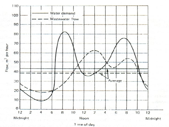
Fluctuations in Rate of Demand • Variations in Water Consumption occur throughout the day, week and season of the year • The average annual water consumption is the total water consumption for the year divided by the number of days per year and the population of the city • There will be a variation in water demand throughout the day, week and the month. The variations area a characteristic of each city and they must be determined by studying water consumption or water pumpage records for the city begin investigated Average Daily Per Capita Demand = Quantity Required in 12 Months/(365 x Population)

Maximum daily flow. The maximum flow rate that occurs over a 24 -hour period based on annual operating data. The maximum daily flow rate is important particularly in the design of facilities involving retention time such as equalization basins and chlorinecontact tanks. Maximum hourly flow. The peak sustained hourly flow rate occurring a 24 -hour period based on annual operating data. Data on peak hourly flows are needed for the design of flow meters, pumping, grit chambers, sedimentation tanks. Minimum daily flow. The minimum daily flow rate that occurs over a 24 -hour period based on annual operating data. Minimum flow rates are important in the sizing of conduits where solid deposition might occur at low flow rates. Minimum hourly flow. Data on the minimum hourly flow rate are needed to determine possible process effects. At some treatment facilities, such as those using trickling filters, recirculation of effluent is required to sustain the process.

• Maximum daily demand = 1. 8 x average daily demand • Maximum hourly demand of maximum day i. e. Peak demand = 1. 5 x avg. hourly demand = 1. 5 x Maximum daily demand/24 = 1. 5 x (1. 8 x avg. daily demand)/24 = 2. 7 x average daily demand/24 = 2. 7 x annual average hourly demand

• Seasonal Variation: Demand peaks during summer. Fire Breakouts are generally more in summer • Daily Variation: depends on the activity. People draw more water on sundays and festival days, thus increasing demand on these days • Hourly variations

Population Forecasting Methods • • Arithmetic Increase Method Geometric Increase Method Incremental Increase Method Decreasing Rate of Growth Method Graphical Comparison with similar cities Ratio Method Logistic Curve Method

Arithmetic Increase Method • Population is assumed to increase at a constant rate. This is the most simple method of population forecast. In this method, the increase in population from decade to decade is assumed constant. The method is used for short- term estimates (1 – 5 yr). Mathematically, Where d. P/dt is the rate of change of population and K is a constant.

The future population is given by Where Pn = future population at the end of n decades P = present population I = average increment for a decade

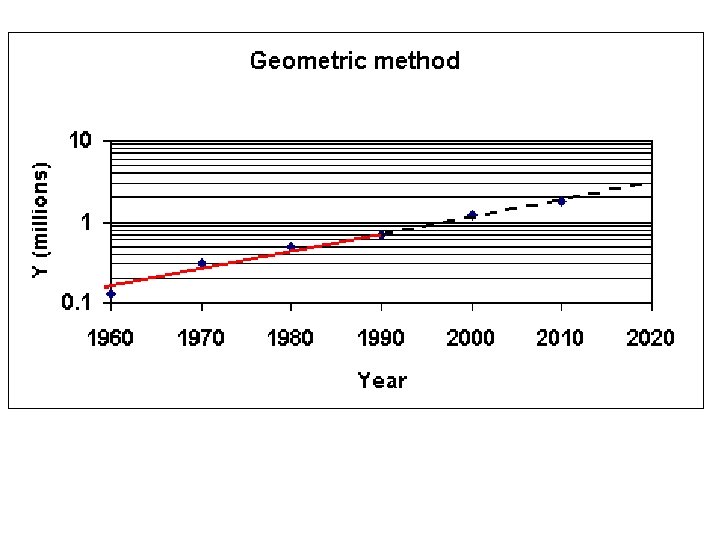
Geometrical Increase Method • Population is assumed to increase in proportion to the number present. i. e. , the percentage increase in population from decade to decade is constant. If Ig is the average percentage increase per decade, or rg is the increase per decade expressed as ratio, the population Pn after n decades is given by

Incremental Increase Method • This method combines both the arithmetic average method and the geometrical average method. Growth rate is assumed to be progressively increasing or decreasing, depending upon whether the average of the incremental increase in the past is positive or negative. The population for a future decade is worked out by adding the mean arithmetic increase to the last known population as in the arithmetic increase method, and to this is added the average of incremental increases, once for first decade, twice for second and so on.

The future population at the end of n decades is given by Where P = present population I = average increase per decade r = average incremental increase n = number of decades

Decreased Rate of Growth Method or Logistic Method • It is found that the rate of increase of population never remains constant, but varies. In this method, the average decrease in the percentage increase is worked out, and is then subtracted from the latest percentage increase to get the percentage increase of next decade.

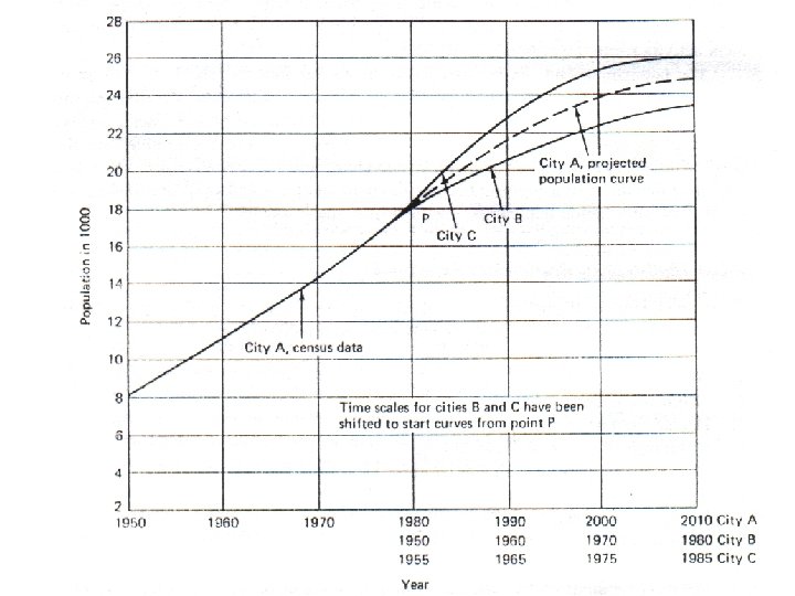
Comparative Graphical Method • In this method, the cities having conditions and characteristics similar to the city whose future population is to be estimated are selected. It is then assumed that the city under consideration will develop, as the selected similar cities have developed in the past.

Ratio Method • In this method, the local population and the country’s population for the last four to five decades is obtained from the census records. The ratios of the local population to national population are then worked out for these decades. A graph is then plotted between time and these ratios, and extended up to the design period to extrapolate the ratio corresponding to future design year. This ratio is then multiplied by the expected national population at the end of the design period, so as to obtain the required city’s future population. Drawbacks: 1. Depends on accuracy of national population estimate 2. Does not consider the abnormal or special conditons which can lead to population shifts from one city to another

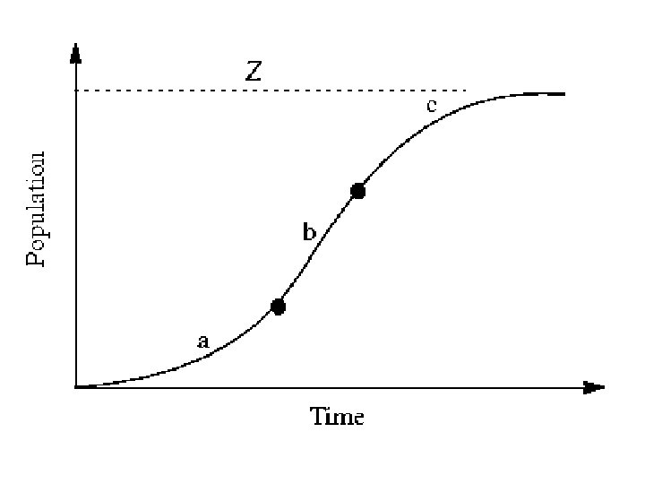
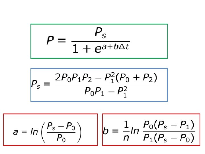
Logistic Curve Method • The three factors responsible for changes in population are: (i) Births (ii) Deaths and (iii) Migrations. Logistic curve method is based on the hypothesis that when these varying influences do not produce extraordinary changes, the population would probably follow the growth curve characteristics of living things within limited space and with limited economic opportunity. The curve is S-shaped and is known as logistic curve.

P = population for a future year Ps = Saturation Population a, b = data constants = future time period, years Po = Population recorded during time to P 1 = Population recorded during time t 1 P 2 = Population recorded at time t 2 The number of years recorded between t 0 and t 1 and t 2 is designated as n.

The logistic method is based on the fact that populations will grow until they reach a saturation population that is established by the limit of economic opportunity. All populations, without regard to size, tend to grow according to the s-shaped curve or logistic curve. The curve starts with a low rate of growth, followed by a high rate, and then by a progressively lower rate until the saturation population is reached

Example: The following is the population data of a city available from past census records. Determine the population of the city in 2011 by (a) arithmetical increase method (b) geometrical increase method © incremental increase method and (d) decreased rate of growth method Year 1931 1941 1951 1961 1971 1981 1991 Population (P) 12000 16500 26800 41500 57500 68000 74100

Year Population Increment per decade % increment per decade 1931 12000 1941 16500 4500 37. 5 1951 26800 10300 62. 42 1961 41500 14700 1971 57500 16000 1981 68000 10500 1991 74100 6100 Total 62100