Water and ecological quality a complex relationship John

Water and ecological quality: a complex relationship John Murray-Bligh UKWIR WW 02 B 029 User Forum Broadway House, London 20 June 2018

Contents Biotic indices RIVPACS RPDS

Relationship between biology and water quality - history in UK Cholera epidemic, Soho 1854 - link disease to water Recognition of importance of aquatic organisms to assess water quality (mainly drinking water) 1870 s Royal Commission 20: 30 standard 1898 -1915 Pearmain, T. H. & C. G. Moore (1899) The analysis of food and drugs Part II chemical and biological analysis of water. London, Ballière, Tindall and Cox The Great Stink - Punch

How do We define environmental quality? What are we trying to protect? Why good status objective? Deviation from reference

We define environmental quality by biology Biology is the main component of environmental quality Provides sustainability – ecosystem services - self-purification Biological quality in freshwater is measured by invertebrates, plants, phytoplankton, fish, diatoms, (and in the future, e. DNA)

Why use biology to quantify water quality? Physico-chemical measures are adequate for managing very polluted water 20/30 standard, smell, visible nuisance Now that serious pollution is resolved, multiple pressures remain as an impacts on biology Biology provides a unified scale for multiple pressures with incompatible scales: water quality - hydrology morphology - alien invasive species. Biology is a more direct measure of what we are trying to protect Natural capital – ecosystem services

Biotic indices Numbers that describe a characteristic of the environment based on biological data Metrics that summarise complex biological data (list of species and abundances) Originally to make biology comprehensible to managers, not for analysing or interpreting results Not amenable to statistical analysis More recently, used to define classification for biological quality objectives and measure quality against them with basic statistical measures

Biotic indices Trait based Empirical Population statistic e. g. total number of species, total abundance, average abundance, evenness of distribution of abundances among species Sensitivity to particular pressure or activity Problems of interpretation – model assumptions Accuracy based on amount of data used to determine sensitivity of each taxon Precision depends on the amount of data used to calculate index (number of taxa) and type of statistic (averages v scores/totals)

Saprobien System (Europe) 1908 -09 + extended eusaprobity xenosaprobity oligosaprobity β-mesosaprobity α-mesosaprobity polysaprobity isosaprobity metasaprobity hypersaprobity ultrasaprobity BOD 5 Index value 0 <1 1 <5 2 <13 3 >20 4 ciliates flagellates bacteria abiotic Biochemical oxygen demand (BOD) mg/l O 2 5 days 20°C

Saprobic index for a site

Succession within limnosaprobity and eusaprobity h Microbial taxa M = mixotrophic phytoflagellates P = producers C = ciliates F = colourless flagellates Z = zooplankton B = bacteria Trophic group producers consumers decomposers s ge a t ls ra rs e uc y t d a bit r o o r r P eb losap t r β e al v n I b uto a ut e o B Z B T te a e r d ter a w sin in ) B B Su r e fac s w r ate ) es B l on ti da gra de n era es g sta s ter a w siv s gre B a fic uri lf-p i F M C F B tio se F C p B m a gs a cre Z Z P α P P x siv Z on ati ic h rop o (pr P ity pro sa s gre e es ity b pro (re te s Wa Saprobic degree h = hypersaprobity m = metasaprobity i = isosaprobity p =polysaprobity α = α-mesosaprobity β = β-mesosaprobity o = oligosaprobity x = xenosaprobity After Sládeček 1973

Impact of sewage effluent Explanation Diagram shows impact of raw sewage discharge and subsequent selfpurification downstream Hynes, 1960

Sensitivity 1. Reduced oxygen 2. Siltation 3. Ammonia toxicity

Other pressures influencing oxygen Low flow Physical modification Canalisation Siltation Eutrophication Oil Phenols/reducing chemicals Thermal discharges Northland Regional Council, NZ Indices sensitive to these pressures will also be sensitive to low oxygen saturation

Saprobity v eutrophy Wegl 1983 saprobity BOD 5 index NH 4 O 2 Trophy mg/l value mg/l oligosaprobic <1 1 <0. 1 >8 oligotrophy β-mesosaprobic <5 2 <0. 5 >6 mesotrohpy α-mesosaprobic <13 3 <13 >2 eutrophy polysaprobic >20 4 >20 <1 hypertrophy total P Chl-a summer biomass mg/m 3 Secchi (m) mg/m 3 <13 <3 >5 <2000 <40 <10 5 -1 >7000 <100 <40 1 -0. 5 <10 000 >100 >40 <0. 5 >10 000 total N mg/m 3 <300 <400 <1000 >1000 Autosaprobity = saprobity generated by biota in the river (by aquatic plants, algae) Allosaprobity = saprobity originating outside the river – allocthonous (leaves, soil run-off, waste) Different aspects of the same thing?

Biological Monitoring Working Party Based on expert’s opinion of sensitivity of families of invertebrates and on Chandler score index Value 1 -10 for every family based on sensitivity Score = Σ values Used 1980 (BMWP-score in National River Quality Survey) 1990 – 2014 (ASPT & Ntaxa used for WFD status classification)

ASPT v N-taxa

WHPT - Walley Hawkes Paisley Trigg Replacement for BMWP indices A refinement of BMWP, based on monitoring data 1990 -2005, taxon scores on same scale as BMWP so ASPTs on same scale Responds to same range of pressures as ASPT Used from 2015 for WFD invertebrate status classification (2 nd cycle river basin management plans)

Why replace BMWP? Better knowledge • e. g. the BMWP had little information about sensitivity of beetles, so gave a value of 5 to all of them • WHPT based on >100, 000 standard samples from the whole UK Better use of data that we already collect (uses abundance and more families) Better compliance with the Water Framework Directive

How WHPT differs from BMWP Separate value for each abundance category of each taxon Modern taxonomy Based on more families • WHPT, 106 taxa • BMWP, 80 taxa WHPT Ntaxa on a different scale to BMWP Ntaxa

Better relationship between dissolved oxygen and BMWP (e. g. small lowland calcareous rivers) WHPT ASPT BMWP ASPT r 2 = 25. 5 r 2 = 47. 5

Natural variation in animals found in different rivers WHPT ASPT 4. 17 WHPT Ntaxa 41. 7 Different natural communities are found in different types of stream Values of biotic indices vary with natural quality as well as the impact of human pressures WHPT ASPT 7. 14 WHPT Ntaxa 21. 4

WFD classification is based on Fractional value of biological metric compared to what it should be in reference conditions • EQR = environmental quality ratio We use RIVPACS model to predict the reference value Concept of reference

Environmental Quality Ratios EQRs If observed = reference, EQR = 1 = reference environmental quality If observed < reference, EQR < 1 = poorer than reference environmental quality

WFD invertebrate status class boundaries Average sensitivity index value Number of different types of invertebrates (taxa) Boundary WHPT ASPT EQR WHPT Ntaxa EQR High/good 0. 97 0. 80 Good/moderate 0. 86 0. 68 Moderate/poor 0. 72 0. 56 Poor/bad 0. 59 0. 47

RIVPACS model RIVPACS = River In. Vertebrate Prediction and Classification System Predicts natural macro-invertebrate fauna from environmental parameters 642 species/groups → genera & families ASPT and N-taxa → ecological classification, probabilities of belonging to quality classes taking account of error and difference in class between two samples Other invertebrate indices Undertakes WFD status classification RICT River Invertebrate Classification Tool Software implementing RIVPACS

RIVPACS Prediction Environmental data → likelihood of capture of: species genera families family abundances → WHPT (& many other indices) for a single season or any combination of seasons spring = March - May summer = June - August autumn = September - November

Environmental data for RIVPACS/RICT Map data Sample data OS grid reference Width Depth Substrate % clay/silt % sand % gravel/pebbles % cobbles/boulders → mean air temperature* → air temperature range* → latitude* → longitude* Altitude Distance from source Slope Discharge or velocity * Calculated by RICT → mean particle size* Geo-chemistry one of: alkalinity calcium total hardness conductivity environmental data must be the norm for site: median of at least 3 -samples collected in different seasons and preferably more than 1 year

RIVPACS IV RICT GB module has 685 reference sites in 43 endgroups + 110 sites in NI

RIVPACS IV GB TWINSPAN classification of natural river invertebrate communities (= end-groups) Confusion! In RICT, the word classification refers only to classification of WFD ecological status Numbers in the body of the dendrogram indicate the number of sites in each group

RIVPACS/RICT prediction Multiple discriminant analysis is used to find the combination of environmental data that most closely replicates the RIVPACS endgroups (classification) of natural biological communities One axis for each environmental variable

Discriminant function discriminates between distributions of the variables, both of which overlap

+ve What is the value of ASPT at site ? Probability of site belonging to Group C C CC C C C C 6. 0 0. 3 0. 4 • Average value of ASPT in each Group -ve d. f. 2 A A A A • • B B 6. 3 0. 2 B B 8. 2 0. 08 discriminant function 1 E E +ve 0. 02 E E E D DD DD D D DD D D • E 5. 3 5. 4 -ve We need to know: average value of index in each Group & probabilities p that site belongs to each Group p (1 -distance from centroid) number of sites in Group

RIVPACS prediction of ASPT Only 5 end-groups A-E shown in this simplified example. RIVPACS IV GB model has 43 end-groups, NI model has 11 end -groups

Suitability (how suitable your site is for the RIVPACS model) Distance of new site to centroid of nearest RIVPACS Group is used as a test of validity of prediction. Suitability codes A warning is given if the probability of belonging to any RIVPACS group is <0. 05 Prediction is abandoned if probability <0. 01

RIVPACS reference sites were best available Not all RIVPACS reference sites were in WFD reference state (next slide. . . )

Flow pressure at RIVPACS III reference sites Larger circle = more unnatural (greater artificial flow pressure) From: Hydrological Regime Classification for WFD by ENTEC

RICT We need to change into Need to change RIVPACS prediction into WFD reference prediction

From best available to WFD reference Two steps: 1. Remove the effect of variation in the quality of RIVPACS reference sites - adjustment 2. Convert the value of prediction to WFD reference state - conversion

Step 1: adjustment to remove effect of variation in the best available quality predicted by RIVPACS Adjust predictions to the High/Good boundary WFD status Bad Poor Moderate RIVPACS prediction adjusted to median EQI of all RIVPACS sites Good High 5 M Distribution of EQI ASPT in RIVPACS II reference sites

Step 2 conversion from high/good to reference WFD status Bad Poor Moderate Adjusted prediction converted from median to reference; adjusted EQI converted to EQR Good High 5 M Distribution of EQI ASPT in RIVPACS II reference sites

Audit of laboratory errors Error affects our measurement of number of taxa Far less effect on ASPT 20 samples audited per lab each year Error in N-taxa is biased because it is easy to miss a taxon when sorting a sample, which doesn’t get recorded, but less easy to record a taxon that is not there. Misidentification and recording errors often involve a loss and gain, so no net effect on N-taxa

Changes in analytical quality The first year that a laboratory is audited it often has poor results. This is typical and also happens with contractors. In 1995 national 5 -yearly survey, some of the ‘improvement’ in environmental quality was actually caused by improved analytical quality. We adjust for bias so that changes in analytical quality are not mistaken for changes in environmental quality.

Bias adjustment for N-taxa Observed Ntaxa 20 Bias + 2 Corrected Ntaxa = 22 Observed data corrected before classification Bias = mean net effect on N-taxa (gains – losses) reported in the Primary audit reports Different bias value was used for each lab each year From 2012, EA uses a global bias value for all its labs Taking bias into account always improves the observed N-taxa and therefore improves the status that is reported. If you don’t adjust for bias, the WFD status will be worse than it should be. The WFD class boundaries assuming bias is taken into account.

Click to e-mail help Always mention RICT in the subject Start

RICT classification report Scroll to see the suitability code and the bias value

UK reference values for river phytobenthos (diatoms) 1 WDS classification metric Trophic diatom Index (TDI) Reference value for TDI = -25. 36 + 56. 83*log 10(alkalinity) – 12. 96*log 10(alkalinity 2) + 3. 21 (Season) Season = 0 (January – June) = 1 (July – December)

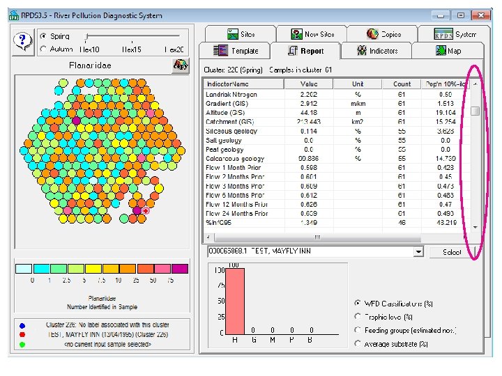
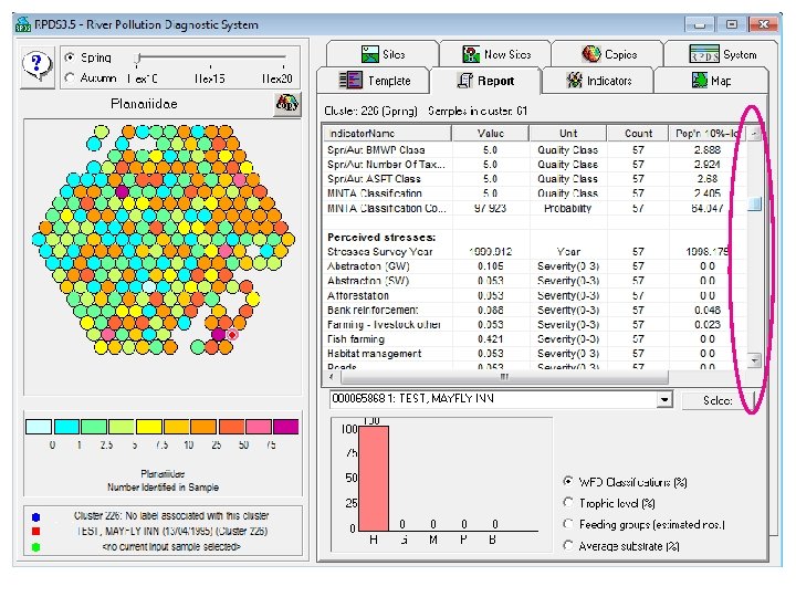
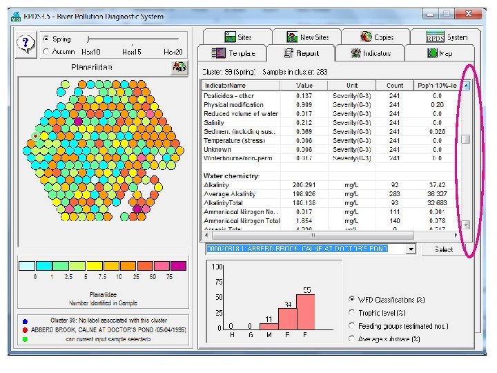
Diagnosis River Pressure Diagnostic System INPUT – biological invertebrate sample data RPDS allocates your biological sample to a cluster of similar biological samples. Each cluster is represented by a circle OUTPUT - diagnosis Average concentrations of chemical, flow or degree of pressure related to samples in a cluster provides the diagnosis for a new biological sample allocated to that cluster. 10 and 90 -percentile ranges allow you to interpret these values as high or low compared to average conditions Artificial intelligence

Aim of RPDS For Water Framework Directive, we must not only classify ecological quality, but also identify the causes of poor quality or degradation so that we can identify an effective programme of measures RPDS helps us diagnose environmental conditions determining the biological quality • If we don’t know what may be causing poor quality • To get a second opinion • To get subjective evidence to support a diagnosis

Conceptual basis of diagnosis Biological community is determined by environmental quality Expert ecologists use two thought processes to interpret biological survey data: pattern-recognition (unsupervised learning based on MIR-max) - RPDS probabilistic reasoning – (Bayesian expert systems) RPBBN From Hynes Biology of Polluted Water

Data used in RPDS V 3. 5 (on EA computer Hydromorphology version network) (stand-alone) Coverage: EA & SEPA More recent data to 2016 Years: 1995 – 2004 (-2016) added (many more samples) Sites: 13, 562 +13, 105 (spring Morphology indices from + autumn) River Habitat Survey such as Biological samples: 85, 626 Habitat Modification Score added 143, 842 Environmental variables: 13 WFD status (WHPT) Chemical determinands: 42 Chemical sites: 5666 (5924) Rectified in updates in 2017 Chemical stats: 3 -yr %ile Perceived stresses (PISCES): 6579 sites RICT predictions WFD status (BMWP) Land cover/use Flow (7367)

MIR-Max Mutual Information and Regression Maximisation Information theory-based MIR-max: allocates biological data to m bins for best performance, then. . . positions bins so that distances between them relate to similarity of data between bins, for better visualisation

Pattern Recognition RPDS display Based on the pattern of abundances of taxa in each sample Similar invertebrate samples are allocated to each bin (also known as a cluster), based on composition and abundance, and selected RIVPACS environmental variables - this stage is know as classification Bins with similar biological samples are closer together Two separate sets of bins: spring Autumn

Open Report tab to view diagnosis of sample or new sample that you have entered Click on cluster to select it in order to show it in report Value = average value in bin = diagnosis Count = number of samples in bin with data = reliability of diagnosis Pop’n 10%ile and 90% - Scroll right to see Pop’n 90%ile These are global statistics based on the mean values in every bin/cluster – different value for spring and autumn Compare with average of samples in bin (value = diagnosis) to see if the value is a particularly high or low

Scrolling down

Indicator = N-taxa Select by double-clicking over chosen indicator Definition of selected indicator

Indicator = ASPT

Indicator = Heptageniidae (intolerant to organic pollution) c. f. ASPT RPDS 3. 2 new photos and text for taxa. Also better explanation of scale. RPDS 3. 3 has text for all indicators Text description for biological indicators includes biology, pollution sensitivity, index values and feeding guild

Boulders occur where slope is greatest - Heptageniidae prefer steeper slope

Boulders occur where slope is greatest - Heptageniidae prefer steeper slope

Summary Sensitivity (WHPT) 4. 17 Number of taxa 41. 7 Sensitivity (WHPT) 7. 14 Number of taxa 21. 4 River Pressure Diagnostic System (RPDS) H River Invertebrate Prediction and Classification System (RIVPACS): 43 natural community types based on 658 samples, predicted from 12 environmental parameters Multivariate analysis: TWINSPAN, multiple discriminant analysis MDA G M P B 255 community types from 72000 biological samples, associated with: 42 chemicals (percentiles from 10 M samples); shading; morphology & habitat (River Habitat Survey, 71 parameters + 12 RIVPACS environmental parameters) flow (7), Land risk analysis (6); perceived stresses (228); Land use (16) Machine learning: Mutual information & regression maximisation Mi. RMax