Warning new jargon Learning jargon is always painful


: “‘Even after the observation of the frequent")
: ‘No free lunch’ for supervised learning: “In a")


 Neural Networks")


")


 between them")


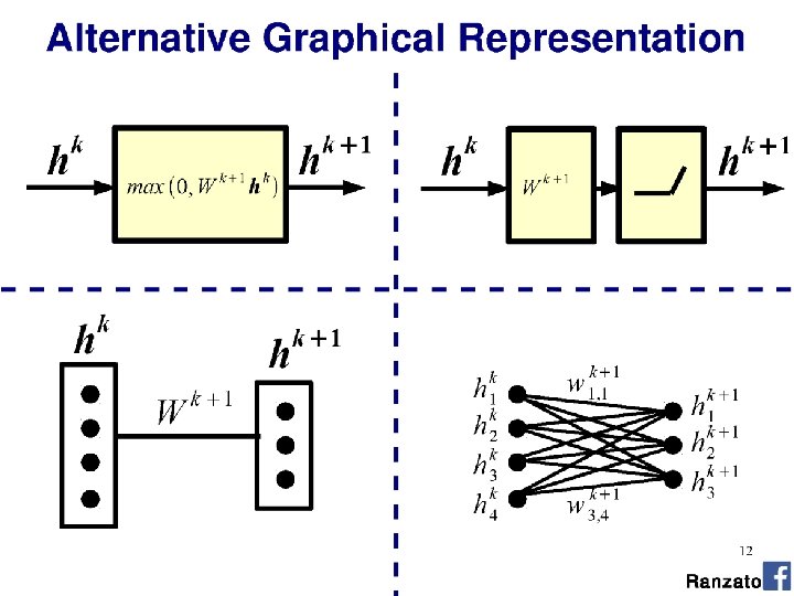
 • …is a ‘fully connected’ neural network with nonlinear activation functions.")


- Slides: 57
Warning – new jargon • Learning jargon is always painful… …even if the concepts behind the jargon are not hard. So, let’s get used to it. “In mathematics you don't understand things. You just get used to them. ” von Neumann (a joke)
Gartner Hype Cycle
Rocket AI
Rocket AI • Launch party @ NIPS 2016 • Neural Information Processing Systems • Academic conference
Rocket AI
Rocket AI Article by Riva-Melissa Tez
Gartner Hype Cycle
So far… Best performing visions systems have commonality: • Hand designed features • Gradients + non-linear operations (exponentiation, clamping, binning) • Features in combination (parts-based models) • Multi-scale representations • Machine learning from databases • Linear classifiers (SVM)
But it’s still not that good… • PASCAL VOC = ~75% • Image. Net = ~75%; human performance = ~95%
Previous claim: It is more important to have more or better labeled data than to use a different supervised learning technique. “The Unreasonable Effectiveness of Data” - Norvig
No free lunch theorem Hume (c. 1739): “‘Even after the observation of the frequent or constant conjunction of objects, we have no reason to draw any inference concerning any object beyond those of which we have had experience. ” -> Learning beyond our experience is impossible.
No free lunch theorem Wolpert (1996): ‘No free lunch’ for supervised learning: “In a noise-free scenario where the loss function is the misclassification rate, if one is interested in offtraining-set error, then there are no a priori distinctions between learning algorithms. ” -> Averaged over all possible datasets, no learning algorithm is better than any other.
OK, well, let’s give up. Class over. No, no! We can build a classifier which better matches the characteristics of the problem!
But…didn’t we just do that? • PASCAL VOC = ~75% • Image. Net = ~75%; human performance = ~95% We used intuition and understanding of how we think vision works, but it still has limitations. Why?
Linear spaces - separability • + kernel trick to transform space. Linearly separable data + linear classifer = good. Kawaguchi
Non-linear spaces - separability • Take XOR – exclusive OR • E. G. , human face has two eyes XOR sunglasses Kawaguchi
Non-linear spaces - separability • Linear functions are insufficient on their own. Kawaguchi
Curse of Dimensionality Every feature that we add requires us to learn the useful regions in a much larger volume. d binary variables = O(2 d) combinations
Curse of Dimensionality • Not all regions of this high-dimensional space are meaningful. >> I = rand(256, 256); >> imshow(I); @ 8 bit = 256 values ^ 65, 536
Related: Manifold Learning locally low-dimensional Euclidean spaces connected and embedded within a high-dim. space. Wikipedia
Local constancy / smoothness of feature space • All existing learning algorithms we have seen assume smoothness or local constancy. -> New example will be near existing examples -> Each region in feature space requires an example Smoothness is ‘averaging’ or ‘interpolating’.
Local constancy / smoothness of feature space • At the extreme: Take k-NN classifier. • The number of regions cannot be more than the number of examples. -> No way to generalize beyond examples How to represent a complex function with more factors than regions?
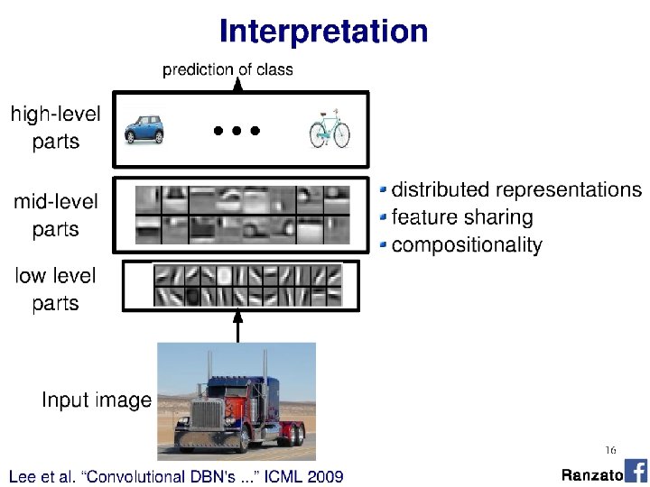
(Deep) Neural Networks
Goals • Build a classifier which is more powerful at representing complex functions and more suited to the learning problem. What does this mean? 1. Assume that the underlying data generating function relies on a composition of factors in a hierarchy. Factor composition = dependencies between regions in feature space.
Example Nielsen, National Geographic
Example Nielsen, National Geographic
Non-linear spaces - separability • Composition of linear functions can represent more complex functions. Kawaguchi
Goals • Build a classifier which is more powerful at representing complex functions and more suited to the learning problem. What does this mean? 2. Learn a feature representation that is specific to the dataset. 10 k/100 k+ data points + factor composition = sophisticated representation.
Neural Networks • Basic building block for composition is a perceptron (Rosenblatt c. 1960) • Linear classifier – vector of weights w and a ‘bias’ b Output (binary)
Binary classifying an image • Each pixel of the image would be an input. • So, for a 28 x 28 image, we vectorize. • x = 1 x 784 • w is a vector of weights for each pixel, 784 x 1 • b is a scalar bias perceptron • result = xw + b -> (1 x 784) x (784 x 1) + b = (1 x 1)+b
Neural Networks - multiclass • Add more perceptrons Binary output
Multi-classifying an image • Each pixel of the image would be an input. • So, for a 28 x 28 image, we vectorize. • x = 1 x 784 • W is a matrix of weights for each pixel/each perceptron • W = 10 x 784 (10 -classification) • b is a bias perceptron (vector of biases); (1 x 10) • result = x. W + b -> (1 x 784) x (784 x 10) + b -> (1 x 10) + (1 x 10) = output vector
Bias convenience • To turn this classification operation into a multiplication only: • Create a ‘fake’ feature with value 1 to represent the bias • Add an extra weight that can vary 1 Output (binary)
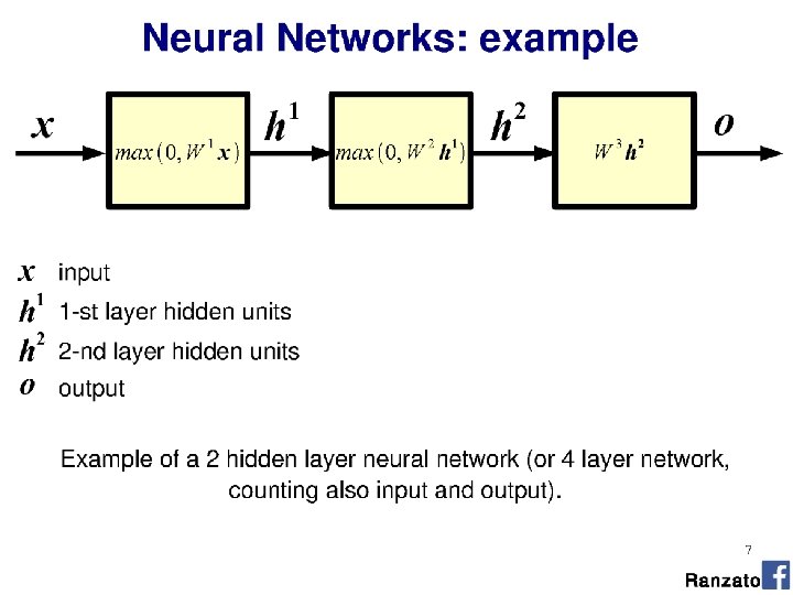
Composition Attempt to represent complex functions as compositions of smaller functions. Outputs from one perception are fed into inputs of another perceptron. Nielsen
Composition Layer 1 Layer 2 Sets of layers and the connections (weights) between them define the network architecture. Nielsen
Composition Hidden Layer 1 Hidden Layer 2 Layers that are in between the input and the output are called hidden layers, because we are going to learn their weights via an optimization process. Nielsen
Composition Hidden Layer 1 Hidden Layer 2 Matrix! Multiple Matrix! It’s all just matrix multiplication! GPUs -> special hardware for fast/large matrix multiplication. Nielsen
Problem 1 with all linear functions • We have formed chains of linear functions. • We know that linear functions can be reduced • g = f(h(x)) • Our composition of functions is really just a single function : (
Problem 2 with all linear functions • Linear classifiers: small change in input can cause large change in binary output. Activation function Nielsen
Problem 2 with all linear functions • Linear classifiers: small change in input can cause large change in binary output. • We want: Nielsen
Let’s introduce non-linearities • We’re going to introduce non-linear functions to transform the features. Nielsen
Rectified Linear Unit • Re. LU
Cyh 24 - http: //prog 3. com/sbdm/blog/cyh_24
Rectified Linear Unit Ranzato
Multi-layer perceptron (MLP) • …is a ‘fully connected’ neural network with nonlinear activation functions. • ‘Feed-forward’ neural network Nielson
MLP • Use is grounded in theory • Universal approximation theorem (Goodfellow 6. 4. 1) • Can represent a NAND circuit, from which any binary function can be built by compositions of NANDs • With enough parameters, it can approximate any function.
Project 6 out today • Good luck finishing project 5! Wei et al.