WARNING 175 slides Print in draft mode 6

WARNING! 175 slides! Print in draft mode, 6 to a page to conserve paper and ink! TR 555 Statistics “Refresher” Lecture 2: Distributions and Tests l l l Binomial, Normal, Log Normal distributions Chi Square and K. S. tests for goodness of fit and independence Poisson and negative exponential Weibull distributions Test Statistics, sample size and Confidence Intervals Hypothesis testing WARNING! 175 slides! Print in draft mode, 6 to a page to conserve paper and ink! 1

Another good reference l 2 http: //www. itl. nist. gov/div 898/handbook/index. htm

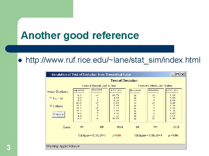
Another good reference l 3 http: //www. ruf. rice. edu/~lane/stat_sim/index. html

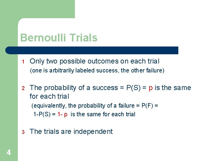
Bernoulli Trials 1 Only two possible outcomes on each trial (one is arbitrarily labeled success, the other failure) 2 The probability of a success = P(S) = p is the same for each trial (equivalently, the probability of a failure = P(F) = 1 -P(S) = 1 - p is the same for each trial 3 4 The trials are independent

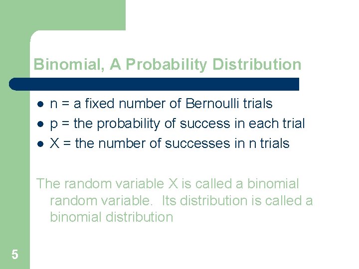
Binomial, A Probability Distribution l l l n = a fixed number of Bernoulli trials p = the probability of success in each trial X = the number of successes in n trials The random variable X is called a binomial random variable. Its distribution is called a binomial distribution 5

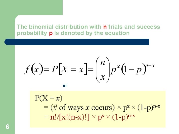
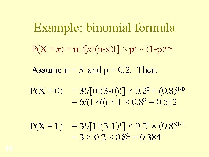
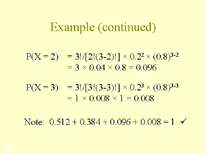
The binomial distribution with n trials and success probability p is denoted by the equation or 6

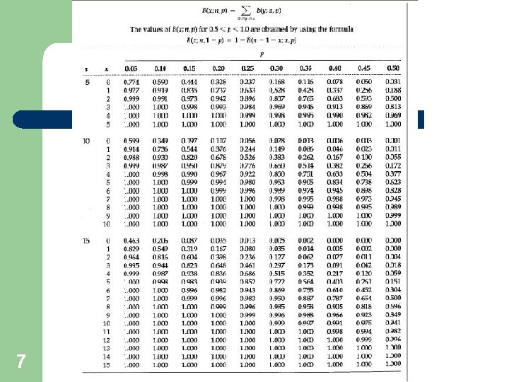
7

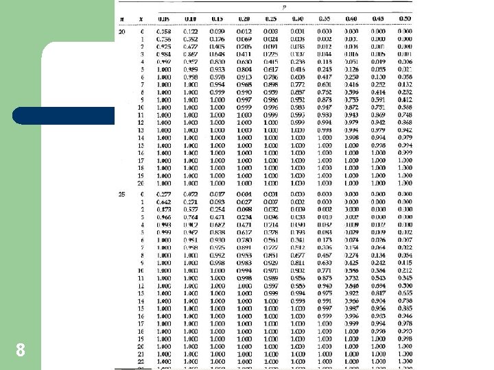
8

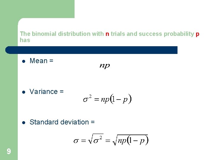
The binomial distribution with n trials and success probability p has 9 l Mean = l Variance = l Standard deviation =

10

11

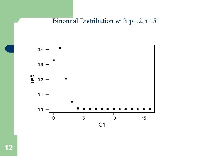
Binomial Distribution with p=. 2, n=5 12

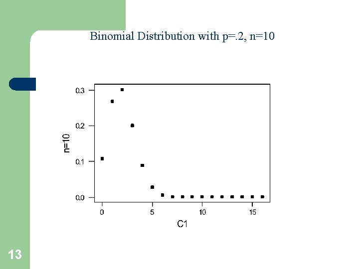
Binomial Distribution with p=. 2, n=10 13

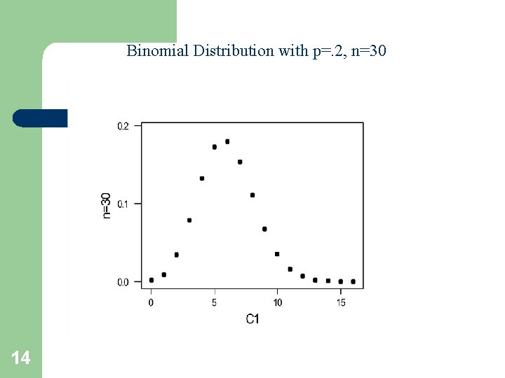
Binomial Distribution with p=. 2, n=30 14

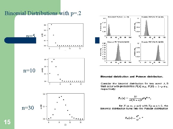
Binomial Distributions with p=. 2 n=5 n=10 n=30 15

Transportation Example l l 16 The probability of making it safely from city A to city B is. 9997 (do we generally know this? ) Traffic per day is 10, 000 trips Assuming independence, what is the probability that there will be more than 3 crashes in a day What is the expected value of the number of crashes?

Transportation Example l l l 17 Expected value = np =. 0003*10000 = 3 P(X>3) = 1 - [P (X=0) + P (X=1) + P (X=2) + P (X=3)] e. g. , P (x=3) = 10000!/(3!*9997!) *. 0003^3 *. 9997^9997 =. 224 don’t just hit 9997! On your calculator! P(X>3) = 1 - [. 050 +. 149 +. 224] = 65%

Continuous probability density functions 18

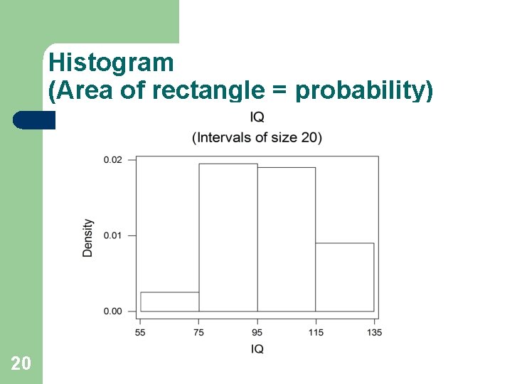
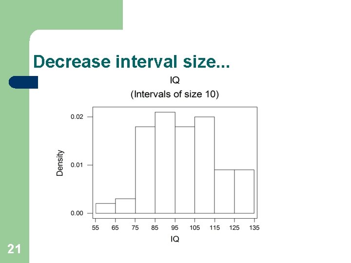
Continuous probability density functions l l 19 The curve describes probability of getting any range of values, say P(X > 120), P(X<100), P(110 < X < 120) Area under the curve = probability Area under whole curve = 1 Probability of getting specific number is 0, e. g. P(X=120) = 0

Histogram (Area of rectangle = probability) 20

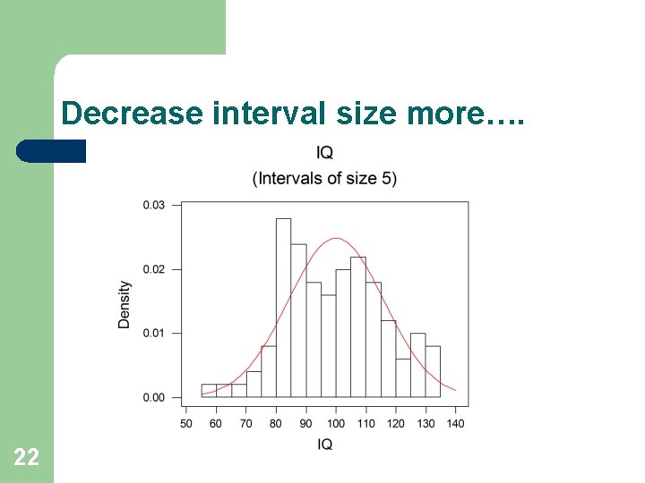
Decrease interval size. . . 21

Decrease interval size more…. 22

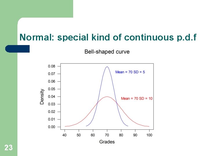
Normal: special kind of continuous p. d. f 23

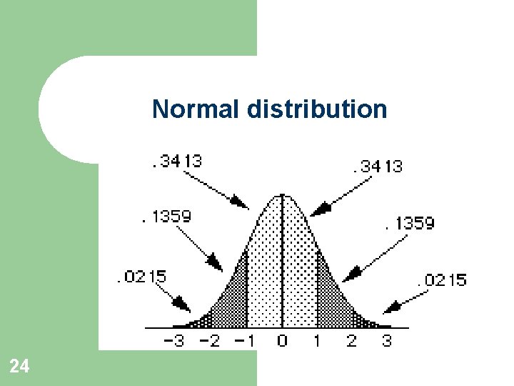
Normal distribution 24

25

Characteristics of normal distribution l l l 26 Symmetric, bell-shaped curve. Shape of curve depends on population mean and standard deviation . Center of distribution is . Spread is determined by . Most values fall around the mean, but some values are smaller and some are larger.

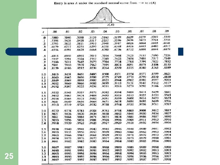
Probability = Area under curve l l 27 Normal integral cannot be solved, so must be numerically integrated - tables We just need a table of probabilities for every possible normal distribution. But there an infinite number of normal distributions (one for each and )!! Solution is to “standardize. ”

Standardizing l l 28 Take value X and subtract its mean from it, and then divide by its standard deviation . Call the resulting value Z. That is, Z = (X- )/ Z is called the standard normal. Its mean is 0 and standard deviation is 1. Then, use probability table for Z.

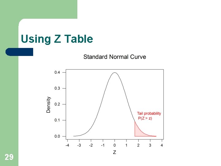
Using Z Table 29

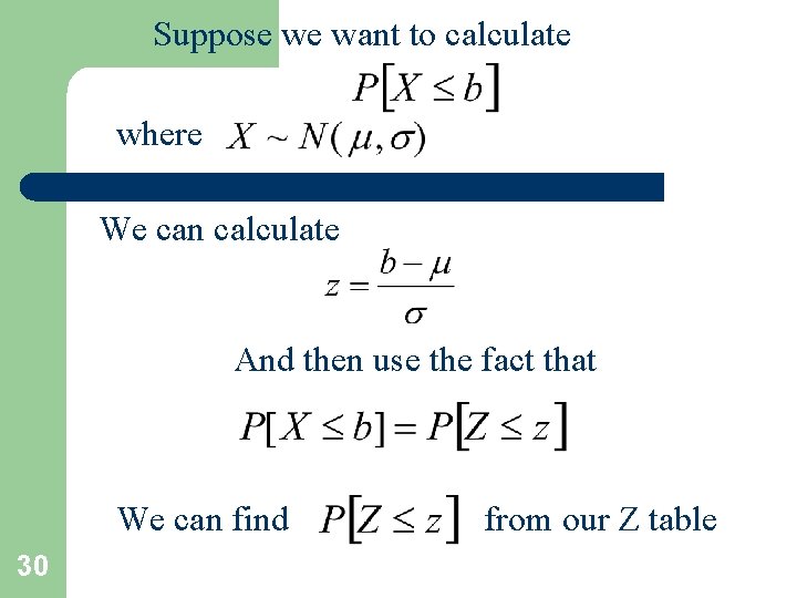
Suppose we want to calculate where We can calculate And then use the fact that We can find 30 from our Z table

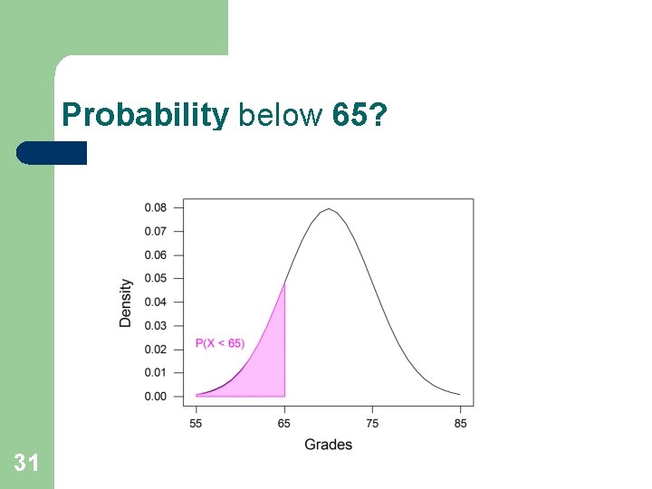
Probability below 65? 31

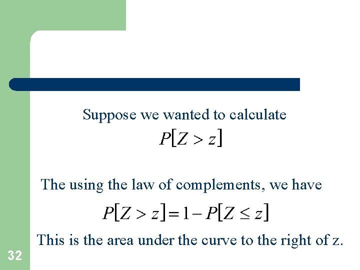
Suppose we wanted to calculate The using the law of complements, we have This is the area under the curve to the right of z. 32

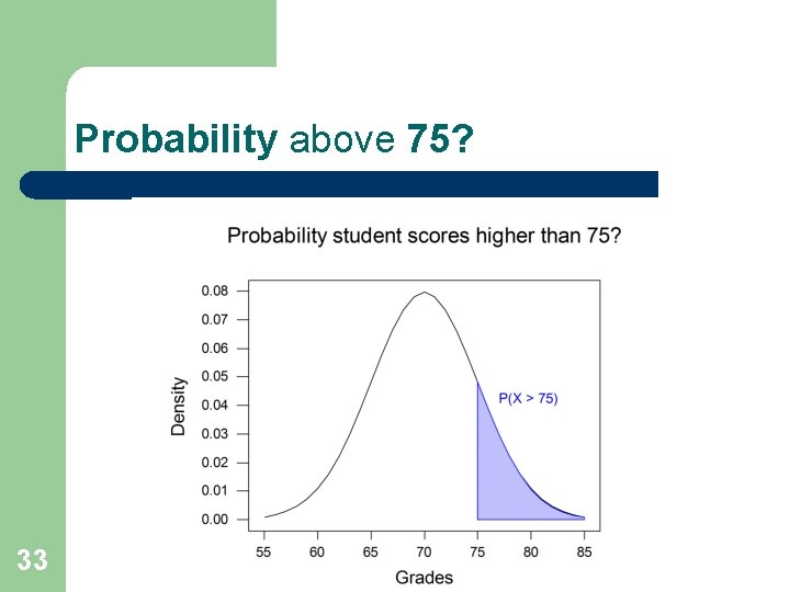
Probability above 75? 33

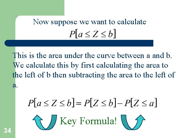
Now suppose we want to calculate This is the area under the curve between a and b. We calculate this by first calculating the area to the left of b then subtracting the area to the left of a. Key Formula! 34

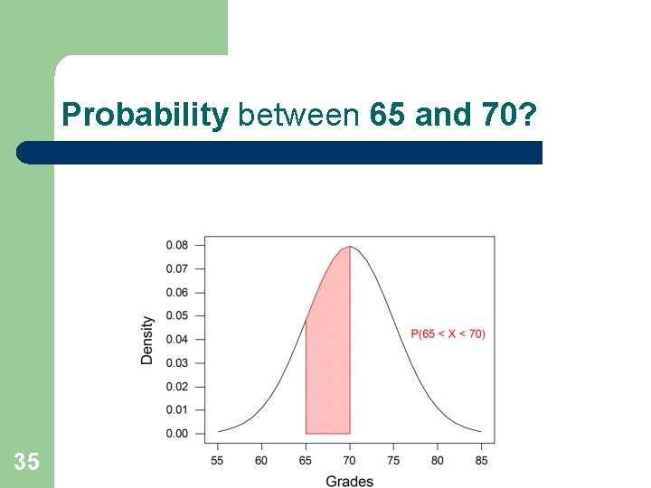
Probability between 65 and 70? 35

Transportation Example l l l 36 Average speeds are thought to be normally distributed Sample speeds are taken, with X = 74. 3 and sigma = 6. 9 What is the speed likely to be exceeded only 5% of the time? Z 95 = 1. 64 (one tail) = (x-74. 3)/6. 9 x = 85. 6 What % are obeying the 75 mph speed limit within a 5 MPH grace?

Assessing Normality l l l 37 the normal distribution requires that the mean is approximately equal to the median, bell shaped, and has the possibility of negative values Histograms Box plots Normal probability plots Chi Square or KS test of goodness of fit

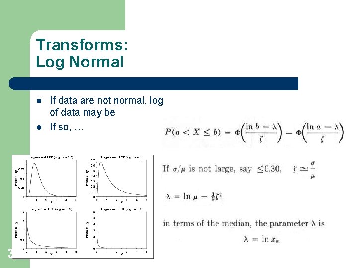
Transforms: Log Normal l l 38 If data are not normal, log of data may be If so, …

39

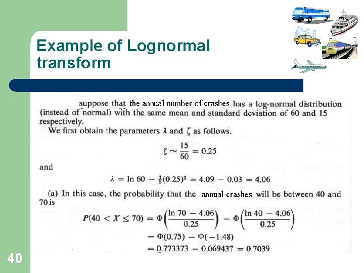
Example of Lognormal transform 40

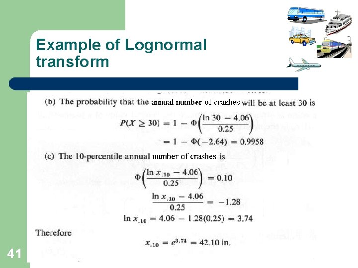
Example of Lognormal transform 41

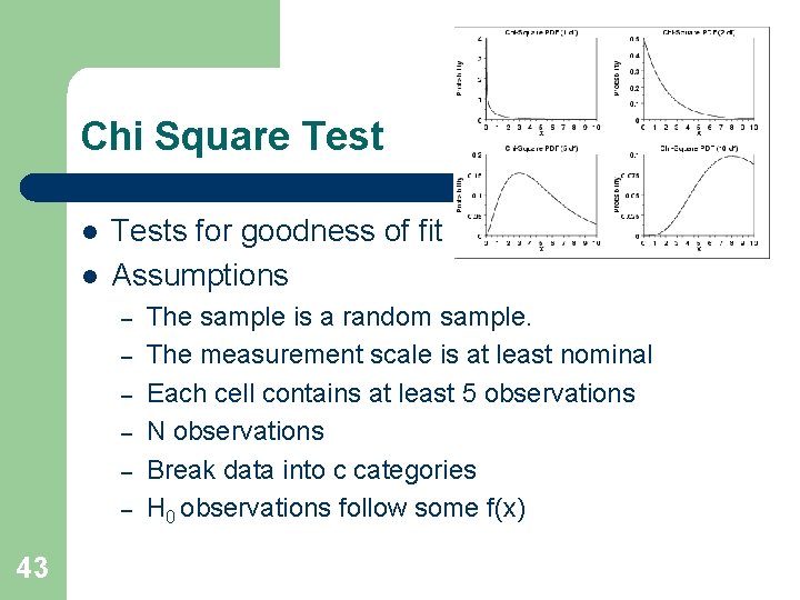
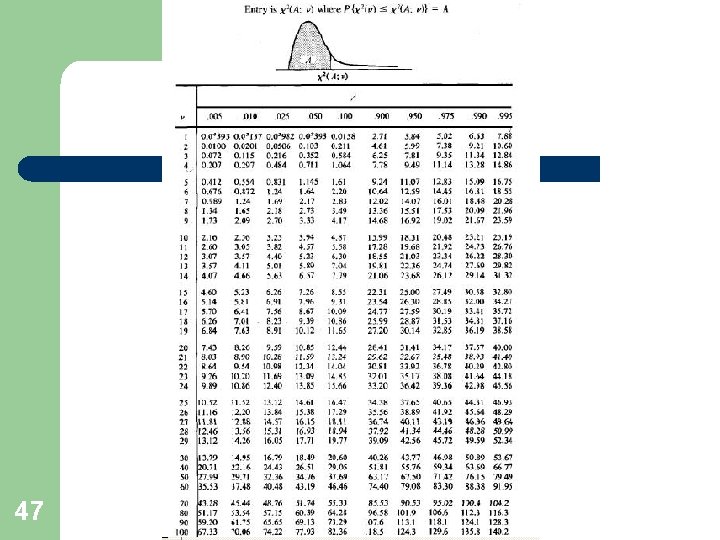
Chi Square Test l l l 42 AKA cross-classification Non-parametric test Use for nominal scale data (or convert your data to nominal scale/categories) Test for normality (or in general, goodness of fit) Test for independence(can also use Cramer’s coefficient for independence or Kendall’s tau for ratio, interval or ordinal data) if used it is important to recognize that it formally applies only to discrete data, the bin intervals chosen influence the outcome, and exact methods (Mehta) provide more reliable results particularly for small sample size

Chi Square Test l l Tests for goodness of fit Assumptions – – – 43 The sample is a random sample. The measurement scale is at least nominal Each cell contains at least 5 observations N observations Break data into c categories H 0 observations follow some f(x)

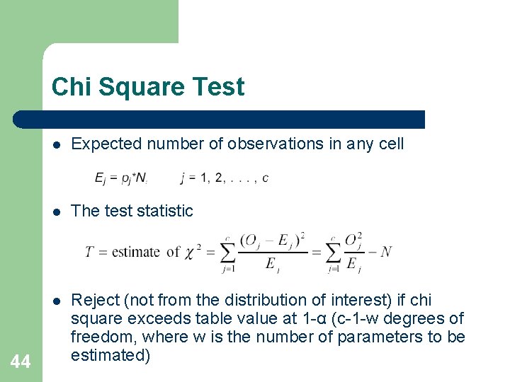
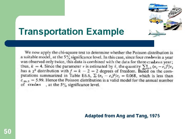
Chi Square Test 44 l Expected number of observations in any cell l The test statistic l Reject (not from the distribution of interest) if chi square exceeds table value at 1 -α (c-1 -w degrees of freedom, where w is the number of parameters to be estimated)

Chi Square Test l l Tests independence of 2 variables Assumptions – – l l 45 N observations R categories for one variable C categories for the other variable At least 5 observations in each cell Prepare an r x c contingency table H 0 the two variables are independent

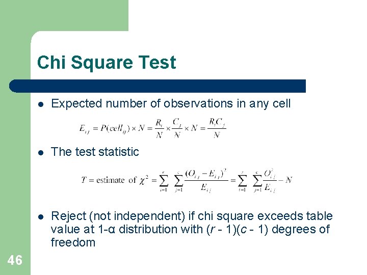
Chi Square Test 46 l Expected number of observations in any cell l The test statistic l Reject (not independent) if chi square exceeds table value at 1 -α distribution with (r - 1)(c - 1) degrees of freedom

47

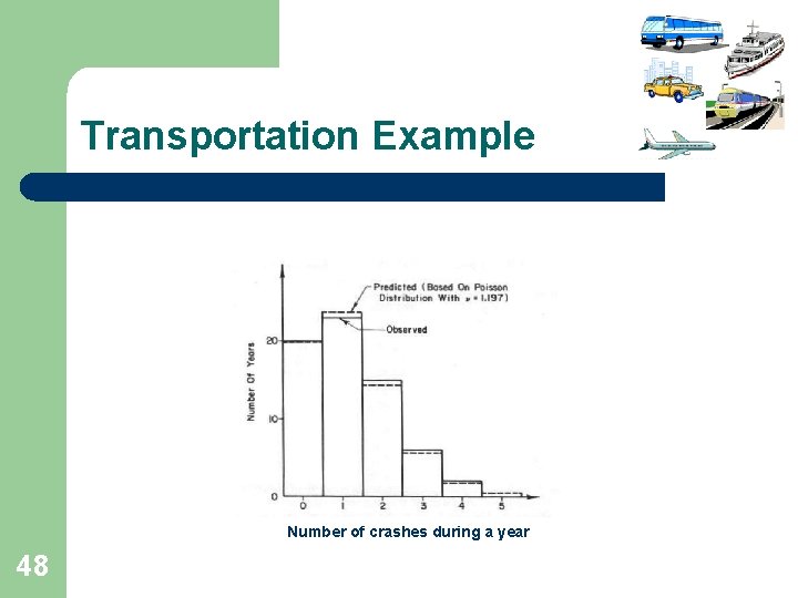
Transportation Example Number of crashes during a year 48

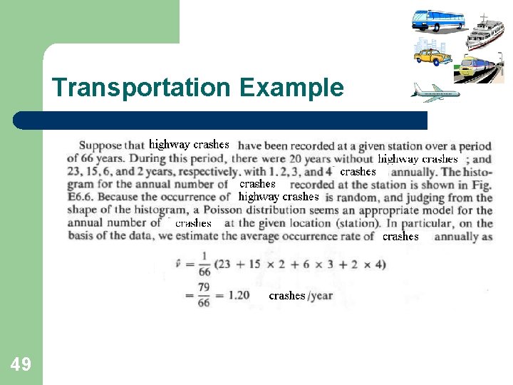
Transportation Example 49

Transportation Example Adapted from Ang and Tang, 1975 50

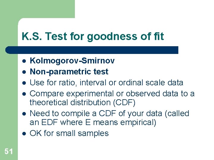
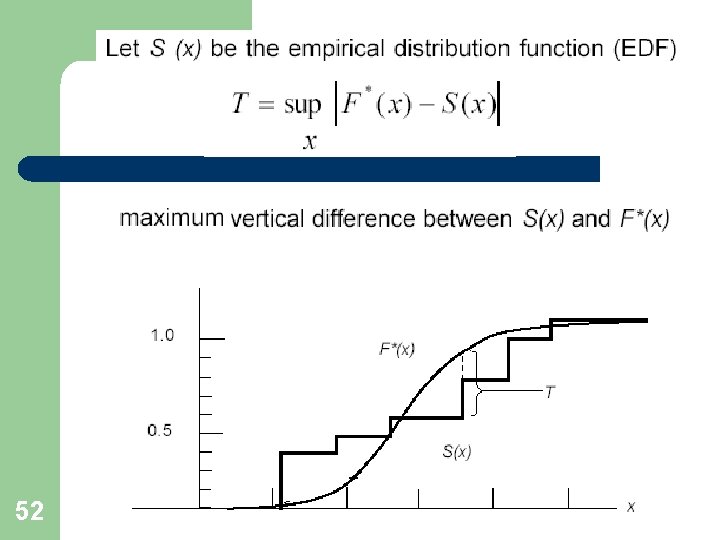
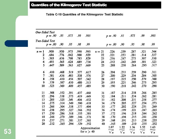
K. S. Test for goodness of fit l l l 51 Kolmogorov-Smirnov Non-parametric test Use for ratio, interval or ordinal scale data Compare experimental or observed data to a theoretical distribution (CDF) Need to compile a CDF of your data (called an EDF where E means empirical) OK for small samples

52

53

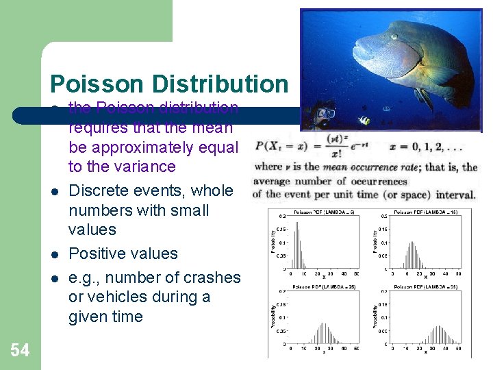
Poisson Distribution l l 54 the Poisson distribution requires that the mean be approximately equal to the variance Discrete events, whole numbers with small values Positive values e. g. , number of crashes or vehicles during a given time

Transportation Example #1 l l 55 On average, 3 crashes per day are experienced on a particular road segment What is the probability that there will be more than 3 crashes in a day

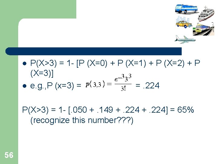
l l P(X>3) = 1 - [P (X=0) + P (X=1) + P (X=2) + P (X=3)] e. g. , P (x=3) = =. 224 P(X>3) = 1 - [. 050 +. 149 +. 224] = 65% (recognize this number? ? ? ) 56

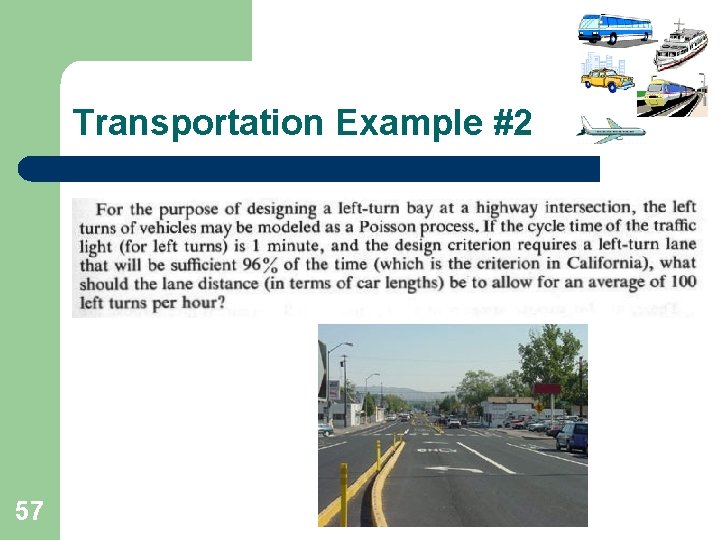
Transportation Example #2 57

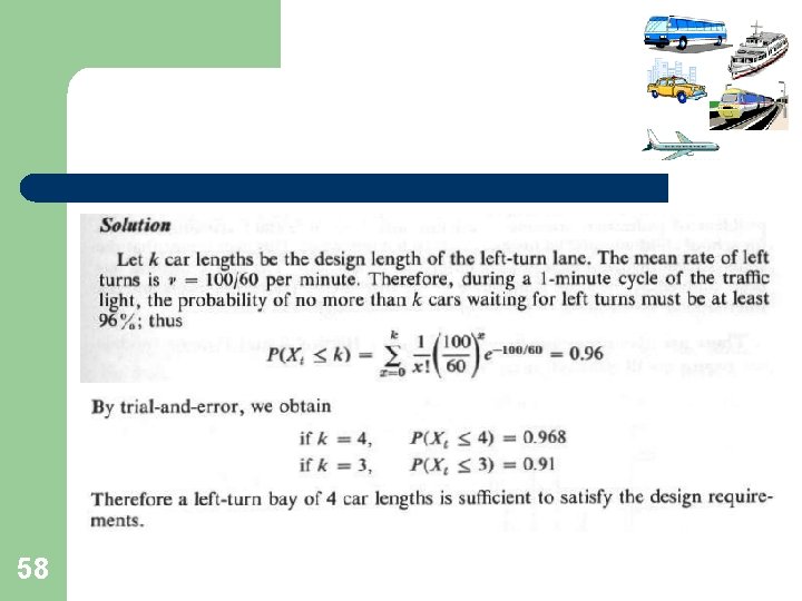
58

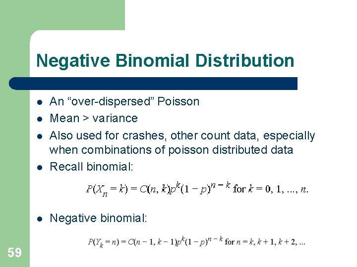
Negative Binomial Distribution l An “over-dispersed” Poisson Mean > variance Also used for crashes, other count data, especially when combinations of poisson distributed data Recall binomial: l Negative binomial: l l l 59

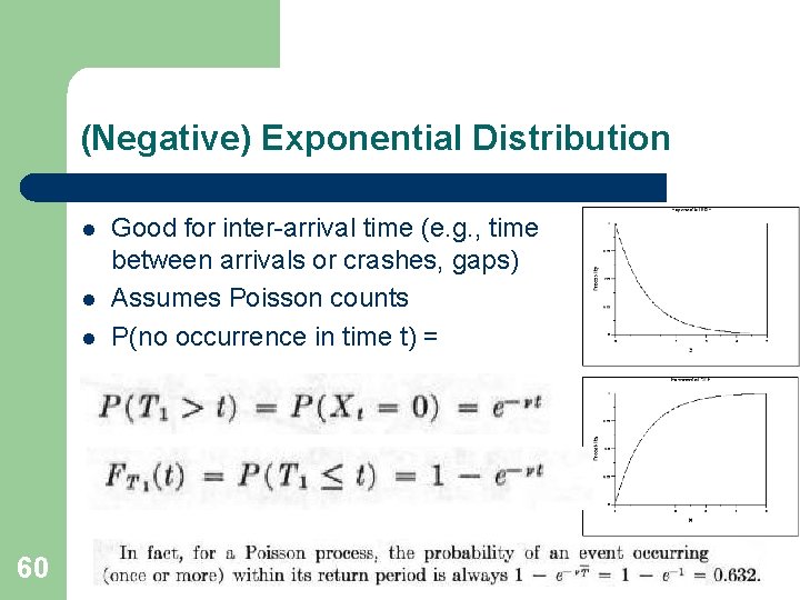
(Negative) Exponential Distribution l l l 60 Good for inter-arrival time (e. g. , time between arrivals or crashes, gaps) Assumes Poisson counts P(no occurrence in time t) =

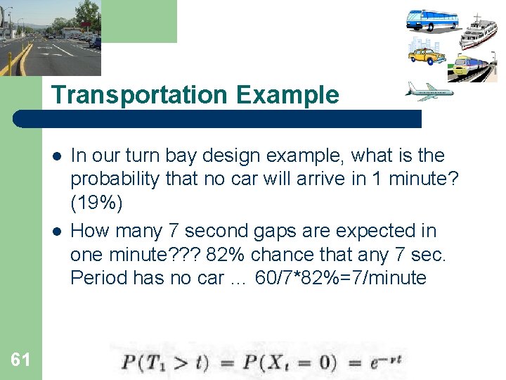
Transportation Example l l 61 In our turn bay design example, what is the probability that no car will arrive in 1 minute? (19%) How many 7 second gaps are expected in one minute? ? ? 82% chance that any 7 sec. Period has no car … 60/7*82%=7/minute

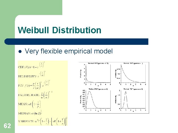
Weibull Distribution l 62 Very flexible empirical model

Sampling Distributions 63

Sampling Distributions l l l 64 Some Definitions Some Common Sense Things An Example A Simulation Sampling Distributions Central Limit Theorem

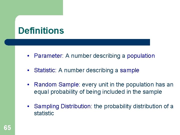
Definitions • Parameter: A number describing a population • Statistic: A number describing a sample • Random Sample: every unit in the population has an equal probability of being included in the sample • Sampling Distribution: the probability distribution of a statistic 65

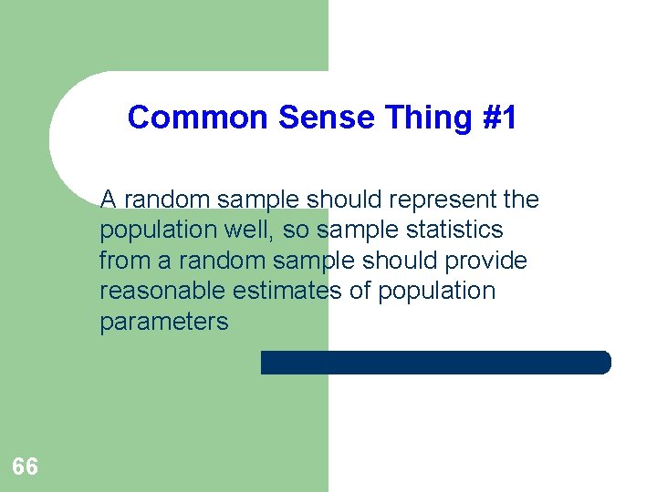
Common Sense Thing #1 A random sample should represent the population well, so sample statistics from a random sample should provide reasonable estimates of population parameters 66

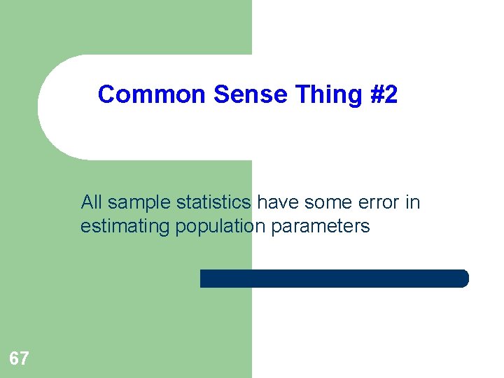
Common Sense Thing #2 All sample statistics have some error in estimating population parameters 67

Common Sense Thing #3 If repeated samples are taken from a population and the same statistic (e. g. mean) is calculated from each sample, the statistics will vary, that is, they will have a distribution 68

Common Sense Thing #4 A larger sample provides more information than a smaller sample so a statistic from a large sample should have less error than a statistic from a small sample 69

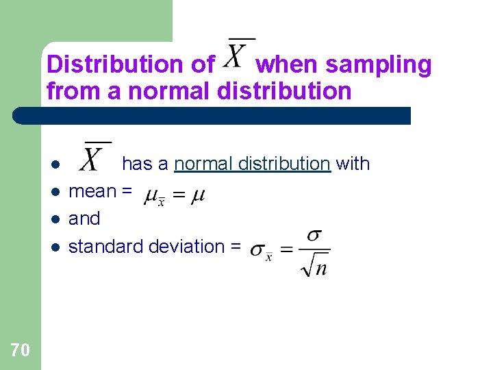
Distribution of when sampling from a normal distribution l l 70 has a normal distribution with mean = and standard deviation =

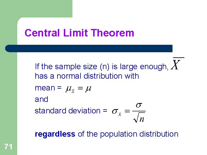
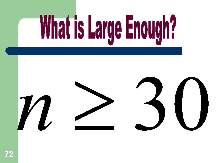
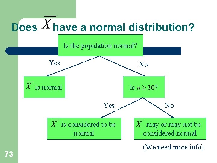
Central Limit Theorem If the sample size (n) is large enough, has a normal distribution with mean = and standard deviation = regardless of the population distribution 71

72

Does have a normal distribution? Is the population normal? Yes No is normal Is Yes is considered to be normal 73 ? No may or may not be considered normal (We need more info)

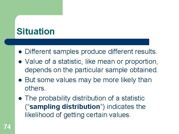
Situation l l 74 Different samples produce different results. Value of a statistic, like mean or proportion, depends on the particular sample obtained. But some values may be more likely than others. The probability distribution of a statistic (“sampling distribution”) indicates the likelihood of getting certain values.

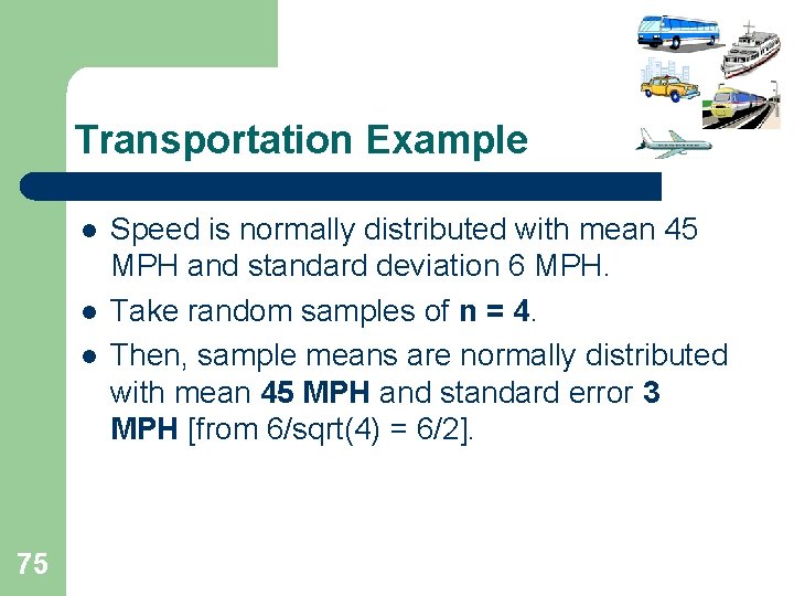
Transportation Example l l l 75 Speed is normally distributed with mean 45 MPH and standard deviation 6 MPH. Take random samples of n = 4. Then, sample means are normally distributed with mean 45 MPH and standard error 3 MPH [from 6/sqrt(4) = 6/2].

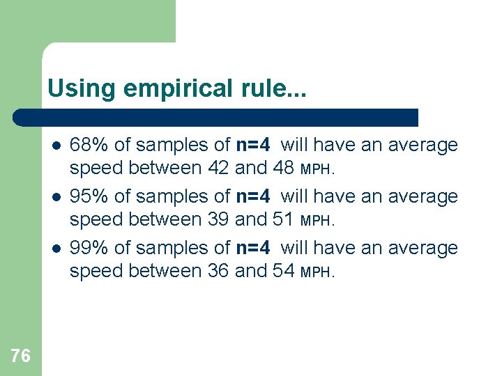
Using empirical rule. . . l l l 76 68% of samples of n=4 will have an average speed between 42 and 48 MPH. 95% of samples of n=4 will have an average speed between 39 and 51 MPH. 99% of samples of n=4 will have an average speed between 36 and 54 MPH.

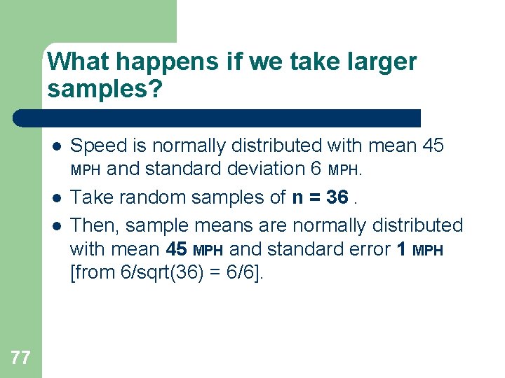
What happens if we take larger samples? l l l 77 Speed is normally distributed with mean 45 MPH and standard deviation 6 MPH. Take random samples of n = 36. Then, sample means are normally distributed with mean 45 MPH and standard error 1 MPH [from 6/sqrt(36) = 6/6].

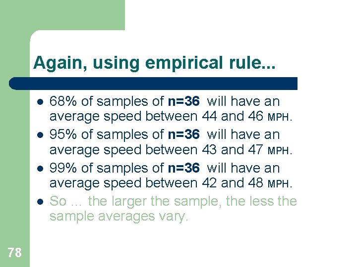
Again, using empirical rule. . . l l 78 68% of samples of n=36 will have an average speed between 44 and 46 MPH. 95% of samples of n=36 will have an average speed between 43 and 47 MPH. 99% of samples of n=36 will have an average speed between 42 and 48 MPH. So … the larger the sample, the less the sample averages vary.

Sampling Distributions for Proportions l l 79 Thought questions Basic rules ESP example Taste test example

Rule for Sample Proportions 80

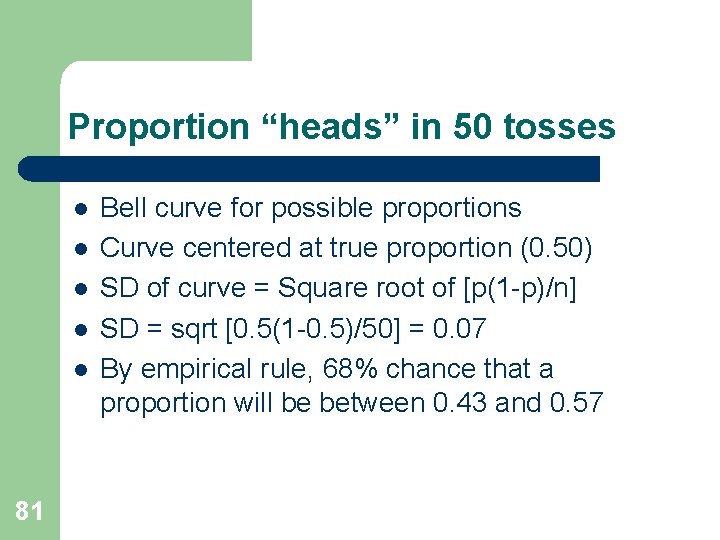
Proportion “heads” in 50 tosses l l l 81 Bell curve for possible proportions Curve centered at true proportion (0. 50) SD of curve = Square root of [p(1 -p)/n] SD = sqrt [0. 5(1 -0. 5)/50] = 0. 07 By empirical rule, 68% chance that a proportion will be between 0. 43 and 0. 57

ESP example l l 82 Five cards are randomly shuffled A card is picked by the researcher Participant guesses which card This is repeated n = 80 times

Many people participate l l l 83 Researcher tests hundreds of people Each person does n = 80 trials The proportion correct is calculated for each person

Who has ESP? l l 84 What sample proportions go beyond luck? What proportions are within the normal guessing range?

Possible results of ESP experiment l l 85 1 in 5 chance of correct guess If guessing, true p = 0. 20 Typical guesser gets p = 0. 20 SD of test = Sqrt [0. 2(1 -0. 2)/80] = 0. 035

Description of possible proportions l l l 86 Bell curve Centered at 0. 2 SD = 0. 035 99% within 0. 095 and 0. 305 (+/- 3 SD) If hundreds of tests, may find several (does it mean they have ESP? )

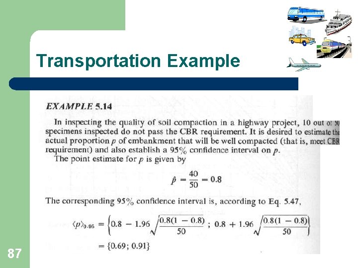
Transportation Example 87

Concepts of Confidence Intervals 88

Confidence Interval l. A range of reasonable guesses at a population value, a mean for instance l. Confidence level = chance that range of guesses captures the population value l. Most common confidence level is 95% 89

General Format of a Confidence Interval lestimate +/- 90 margin of error

Transportation Example: Accuracy of a mean l. A sample of n=36 has mean speed = 75. 3. l. The SD = 8. l. How well does this sample mean estimate the population mean ? 91

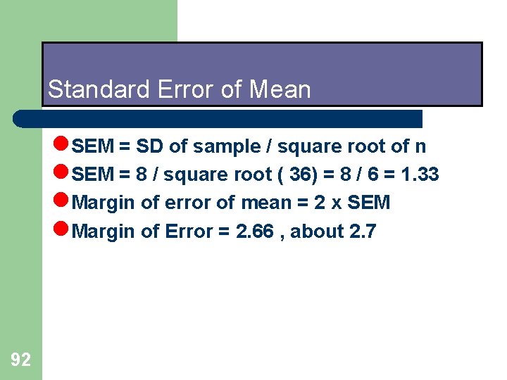
Standard Error of Mean l. SEM = SD of sample / square root of n l. SEM = 8 / square root ( 36) = 8 / 6 = 1. 33 l. Margin of error of mean = 2 x SEM l. Margin of Error = 2. 66 , about 2. 7 92

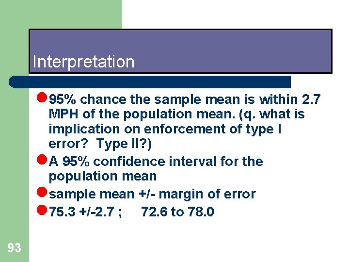
Interpretation l 95% chance the sample mean is within 2. 7 MPH of the population mean. (q. what is implication on enforcement of type I error? Type II? ) l. A 95% confidence interval for the population mean lsample mean +/- margin of error l 75. 3 +/-2. 7 ; 72. 6 to 78. 0 93

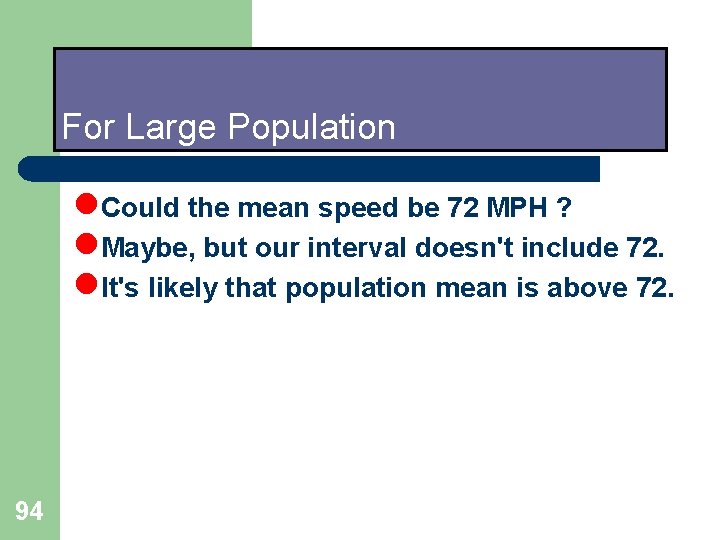
For Large Population l. Could the mean speed be 72 MPH ? l. Maybe, but our interval doesn't include 72. l. It's likely that population mean is above 72. 94

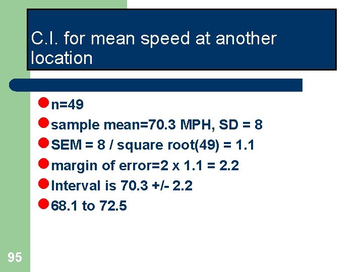
C. I. for mean speed at another location ln=49 lsample mean=70. 3 MPH, SD = 8 l. SEM = 8 / square root(49) = 1. 1 lmargin of error=2 x 1. 1 = 2. 2 l. Interval is 70. 3 +/- 2. 2 l 68. 1 to 72. 5 95

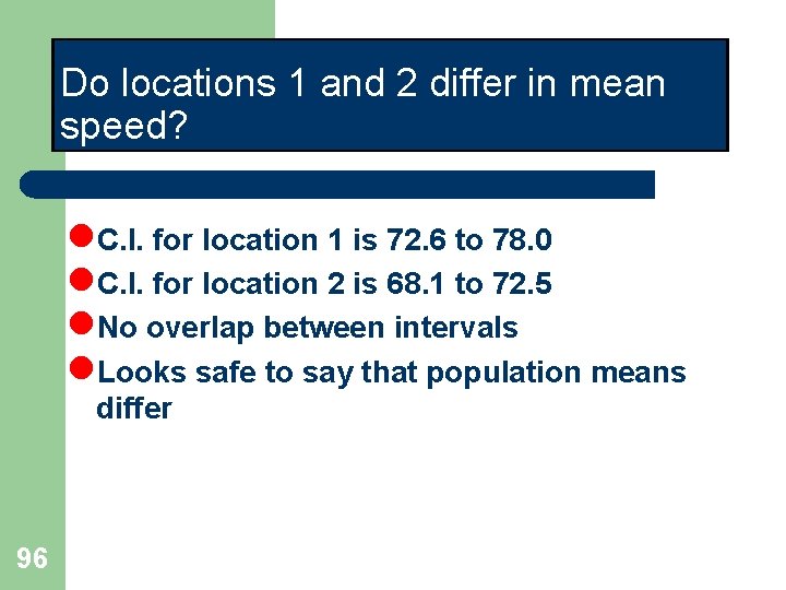
Do locations 1 and 2 differ in mean speed? l. C. I. for location 1 is 72. 6 to 78. 0 l. C. I. for location 2 is 68. 1 to 72. 5 l. No overlap between intervals l. Looks safe to say that population means differ 96

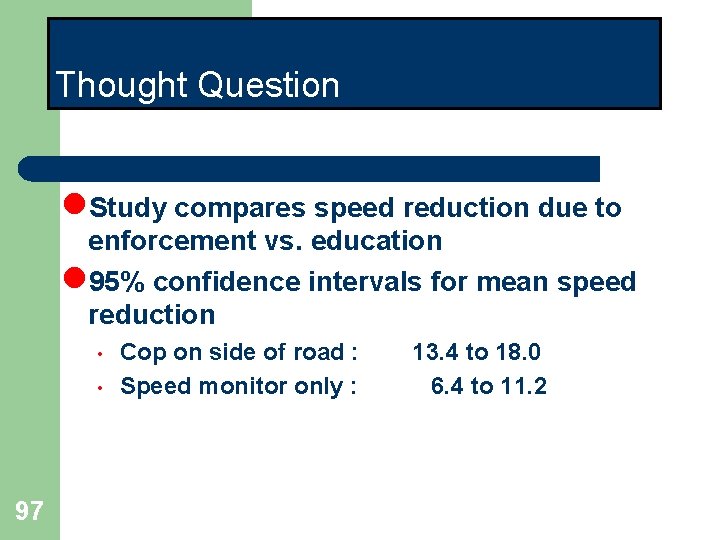
Thought Question l. Study compares speed reduction due to enforcement vs. education l 95% confidence intervals for mean speed reduction • • 97 Cop on side of road : Speed monitor only : 13. 4 to 18. 0 6. 4 to 11. 2

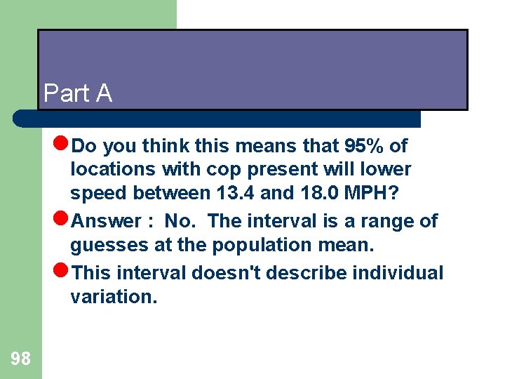
Part A l. Do you think this means that 95% of locations with cop present will lower speed between 13. 4 and 18. 0 MPH? l. Answer : No. The interval is a range of guesses at the population mean. l. This interval doesn't describe individual variation. 98

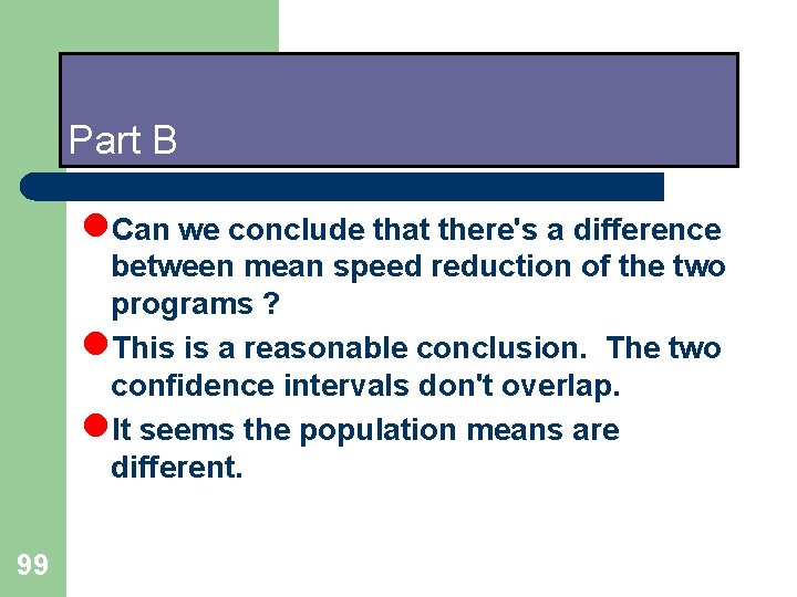
Part B l. Can we conclude that there's a difference between mean speed reduction of the two programs ? l. This is a reasonable conclusion. The two confidence intervals don't overlap. l. It seems the population means are different. 99

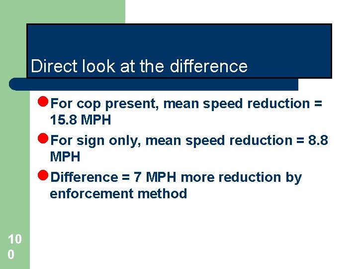
Direct look at the difference l. For cop present, mean speed reduction = 15. 8 MPH l. For sign only, mean speed reduction = 8. 8 MPH l. Difference = 7 MPH more reduction by enforcement method 10 0

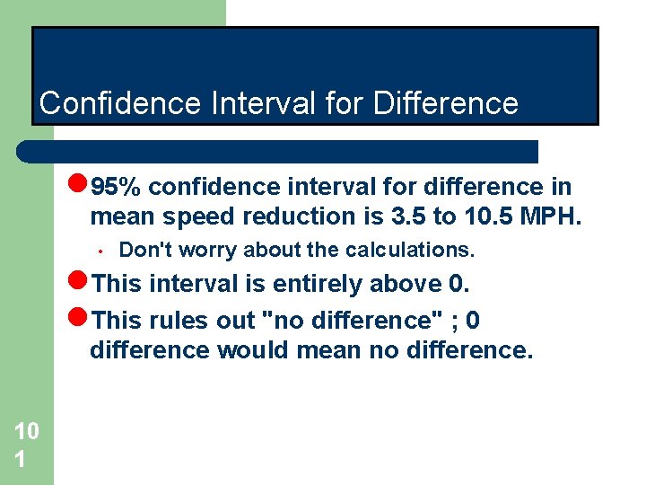
Confidence Interval for Difference l 95% confidence interval for difference in mean speed reduction is 3. 5 to 10. 5 MPH. • Don't worry about the calculations. l. This interval is entirely above 0. l. This rules out "no difference" ; 0 difference would mean no difference. 10 1

Confidence Interval for a Mean when you have a “small” sample. . . 10 2

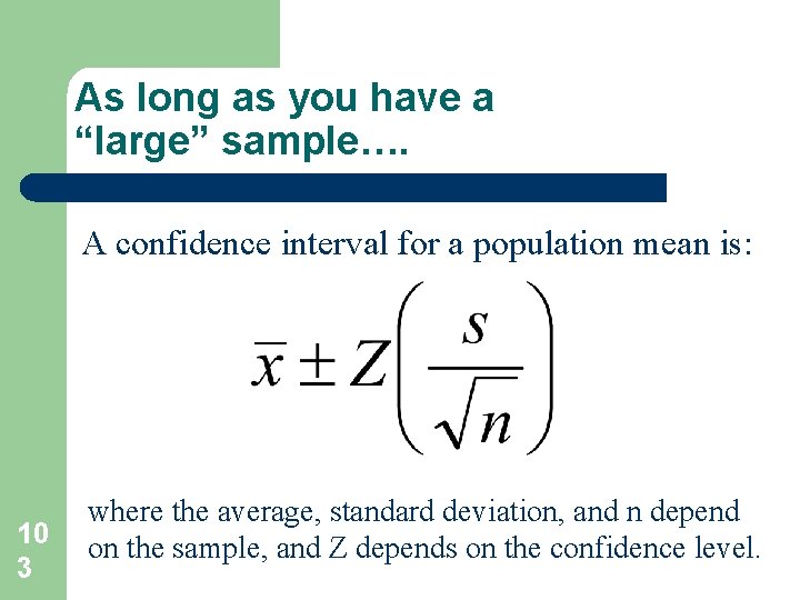
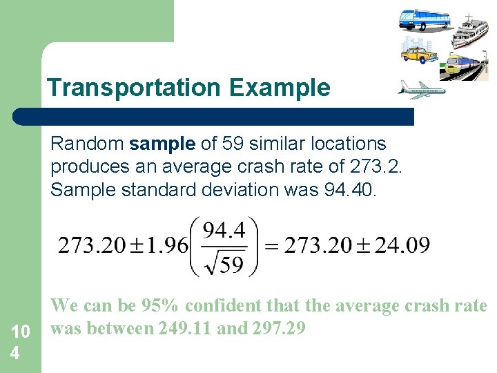
As long as you have a “large” sample…. A confidence interval for a population mean is: 10 3 where the average, standard deviation, and n depend on the sample, and Z depends on the confidence level.

Transportation Example Random sample of 59 similar locations produces an average crash rate of 273. 2. Sample standard deviation was 94. 40. 10 4 We can be 95% confident that the average crash rate was between 249. 11 and 297. 29

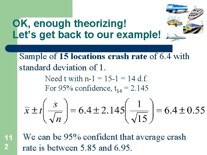
What happens if you can only take a “small” sample? l l 10 5 Random sample of 15 similar location crash rates had an average of 6. 4 with standard deviation of 1. What is the average crash rate at all similar locations?

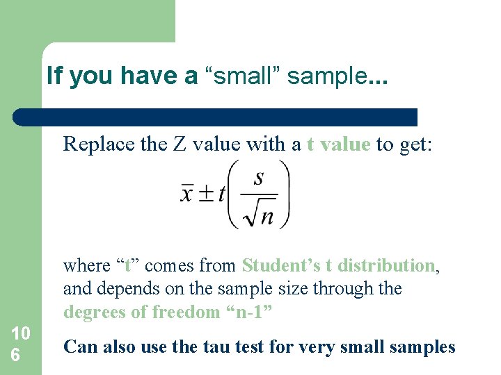
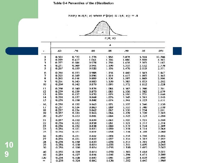
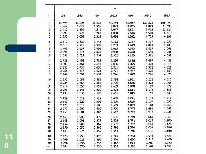
If you have a “small” sample. . . Replace the Z value with a t value to get: where “t” comes from Student’s t distribution, and depends on the sample size through the degrees of freedom “n-1” 10 6 Can also use the tau test for very small samples

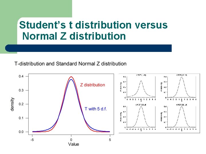
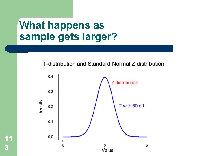
Student’s t distribution versus Normal Z distribution 10 7

T distribution l l l 10 8 Very similar to standard normal distribution, except: t depends on the degrees of freedom “n-1” more likely to get extreme t values than extreme Z values

10 9

11 0

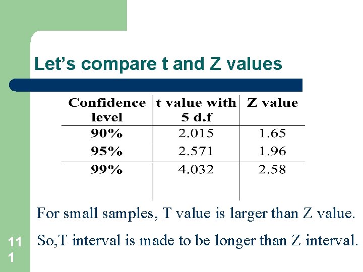
Let’s compare t and Z values For small samples, T value is larger than Z value. 11 1 So, T interval is made to be longer than Z interval.

OK, enough theorizing! Let’s get back to our example! Sample of 15 locations crash rate of 6. 4 with standard deviation of 1. Need t with n-1 = 15 -1 = 14 d. f. For 95% confidence, t 14 = 2. 145 11 2 We can be 95% confident that average crash rate is between 5. 85 and 6. 95.

What happens as sample gets larger? 11 3

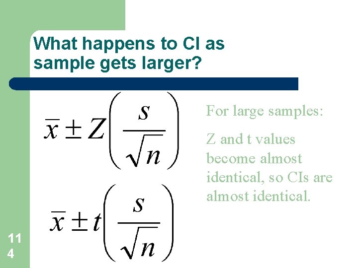
What happens to CI as sample gets larger? For large samples: Z and t values become almost identical, so CIs are almost identical. 11 4

One not-so-small problem! l l 11 5 It is only OK to use the t interval for small samples if your original measurements are normally distributed. We’ll learn how to check for normality in a minute.

Strategy for deciding how to analyze l l l 11 6 If you have a large sample of, say, 60 or more measurements, then don’t worry about normality, and use the z-interval. If you have a small sample and your data are normally distributed, then use the t-interval. If you have a small sample and your data are not normally distributed, then do not use the t -interval, and stay tuned for what to do.

Hypothesis tests l Test should begin with a set of specific, testable hypotheses that can be tested using data: Not a meaningful hypothesis – Was safety improved by improvements to roadway – Meaningful hypothesis – Were speeds reduced when traffic calming was introduced. – Usually to demonstrate evidence that there is a difference in measurable quantities l Hypothesis testing is a decision-making tool. l 11 7

Hypothesis Step 1 l Provide one working hypothesis – the null hypothesis – and an alternative l The null or nil hypothesis convention is generally that nothing happened – Example l speeds were not reduced after traffic calming – Null Hypothesis l Speed were reduced after traffic calming – Alternative Hypothesis l When stating the hypothesis, the analyst must think of the impact of the potential error. 11 8

Step 2, select appropriate statistical test l The analyst may wish to test – Changes in the mean of events – Changes in the variation of events – Changes in the distribution of events 11 9

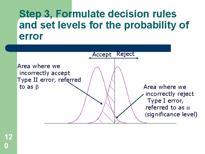
Step 3, Formulate decision rules and set levels for the probability of error Accept Reject Area where we incorrectly accept Type II error, referred to as b 12 0 Area where we incorrectly reject Type I error, referred to as (significance level)

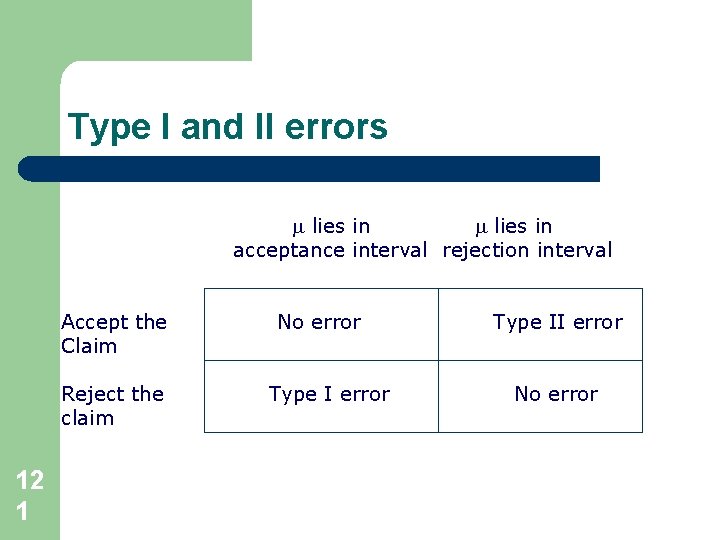
Type I and II errors lies in acceptance interval rejection interval Accept the Claim Reject the claim 12 1 No error Type II error No error

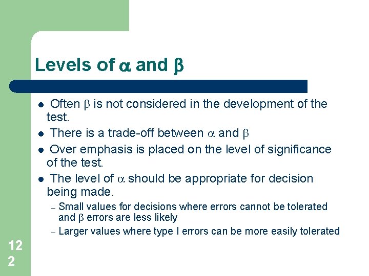
Levels of and b Often b is not considered in the development of the test. l There is a trade-off between and b l Over emphasis is placed on the level of significance of the test. l The level of should be appropriate for decision being made. l Small values for decisions where errors cannot be tolerated and b errors are less likely – Larger values where type I errors can be more easily tolerated – 12 2

Step 4 Check statistical assumption l Draw new samples to check answer l Check the following assumption – Are data continuous or discrete – Plot data – Inspect to make sure that data meets assumptions l For example, the normal distribution assumes that mean = median – Inspect 12 3 results for reasonableness

Step 5 Make decision l Typical misconceptions – Alpha is the most important error – Hypothesis tests are unconditional l It does not provide evidence that the working hypothesis is true – Hypothesis test conclusion are correct l Assume 300 independent tests – 100 rejection of work hypothesis – = 0. 05 and b = 0. 10 – Thus 0. 05 x 100 = 5 Type I errors – And 0. 1 x 200 = 20 Type II errors – 25 time out of 300 the test results were wrong – 12 4

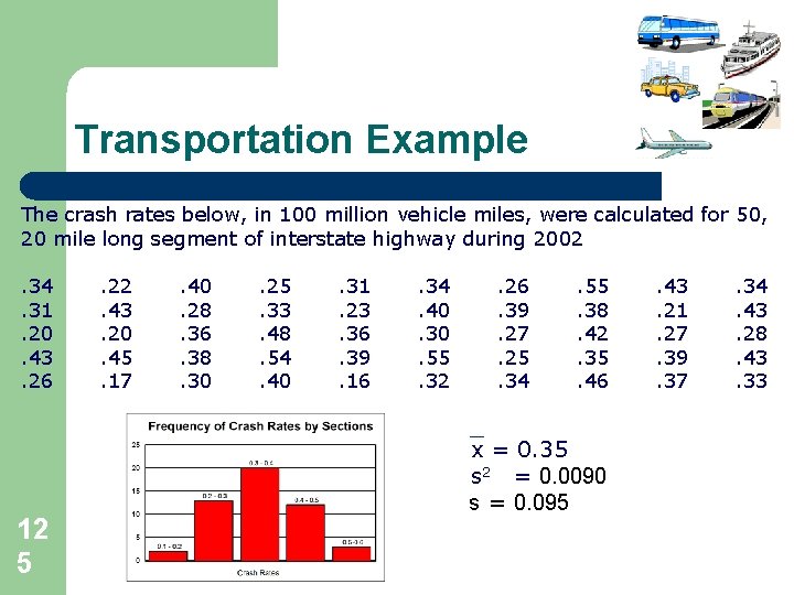
Transportation Example The crash rates below, in 100 million vehicle miles, were calculated for 50, 20 mile long segment of interstate highway during 2002. 34. 31. 20. 43. 26 12 5 . 22. 43. 20. 45. 17 . 40. 28. 36. 38. 30 . 25. 33. 48. 54. 40 . 31. 23. 36. 39. 16 . 34. 40. 30. 55. 32 . 26. 39. 27. 25. 34 . 55. 38. 42. 35. 46 x = 0. 35 s 2 = 0. 0090 s = 0. 095 . 43. 21. 27. 39. 37 . 34. 43. 28. 43. 33

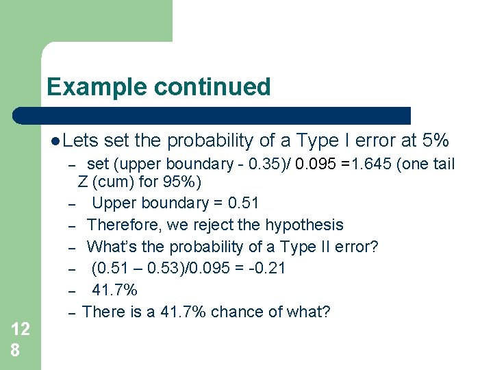
Example continued Crash rates are collected from non-interstate system highways built to slightly lower design standards. Similarly and average crash rate is calculated and it is greater (0. 53). Also assume that both means have the same standard deviation (0. 095). The question is do we arrive at the same accident rate with both facilities. Our hypothesis is that both have the same means f = nf Can we accept or reject our hypothesis? 12 6

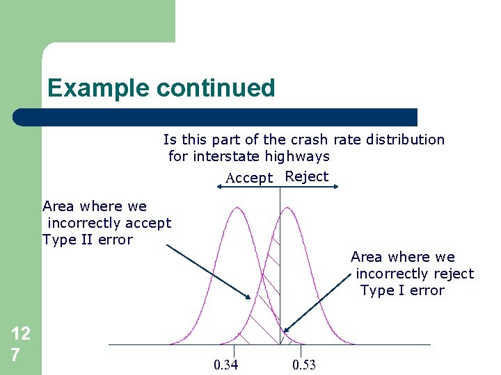
Example continued Is this part of the crash rate distribution for interstate highways Accept Reject Area where we incorrectly accept Type II error Area where we incorrectly reject Type I error 12 7 0. 34 0. 53

Example continued l Lets set (upper boundary - 0. 35)/ 0. 095 =1. 645 (one tail Z (cum) for 95%) – Upper boundary = 0. 51 – Therefore, we reject the hypothesis – What’s the probability of a Type II error? – (0. 51 – 0. 53)/0. 095 = -0. 21 – 41. 7% – There is a 41. 7% chance of what? – 12 8 set the probability of a Type I error at 5%

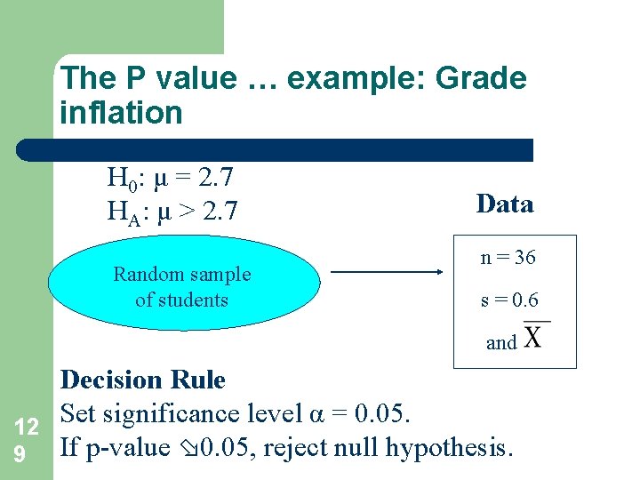
The P value … example: Grade inflation H 0: μ = 2. 7 HA: μ > 2. 7 Random sample of students Data n = 36 s = 0. 6 and Decision Rule Set significance level α = 0. 05. 12 9 If p-value 0. 05, reject null hypothesis.

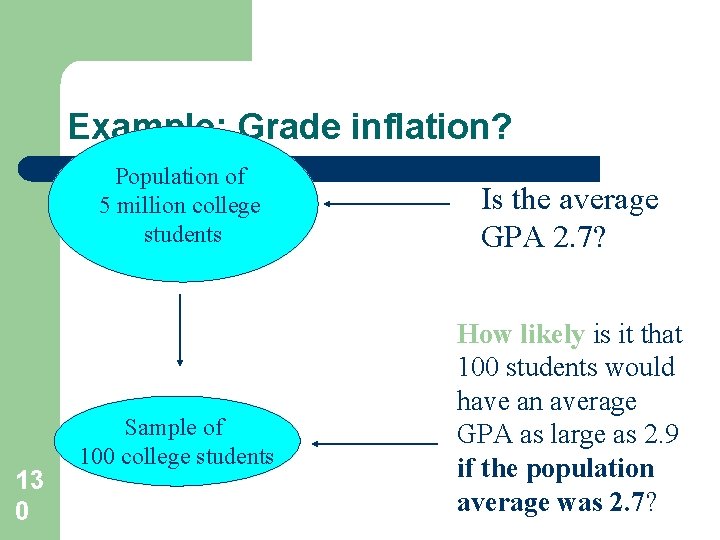
Example: Grade inflation? Population of 5 million college students 13 0 Sample of 100 college students Is the average GPA 2. 7? How likely is it that 100 students would have an average GPA as large as 2. 9 if the population average was 2. 7?

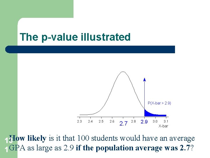
The p-value illustrated How likely is it that 100 students would have an average 13 1 GPA as large as 2. 9 if the population average was 2. 7?

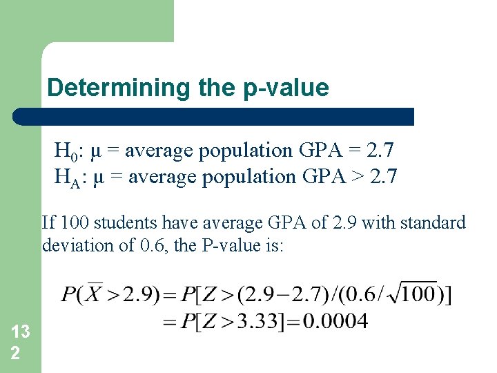
Determining the p-value H 0: μ = average population GPA = 2. 7 HA: μ = average population GPA > 2. 7 If 100 students have average GPA of 2. 9 with standard deviation of 0. 6, the P-value is: 13 2

Making the decision l l 13 3 The p-value is “small. ” It is unlikely that we would get a sample as large as 2. 9 if the average GPA of the population was 2. 7. Reject H 0. There is sufficient evidence to conclude that the average GPA is greater than 2. 7.

Terminology l l l 13 4 H 0: μ = 2. 7 versus HA: μ > 2. 7 is called a “right-tailed” or a “one-sided” hypothesis test, since the p-value is in the right tail. Z = 3. 33 is called the “test statistic”. If we think our p-value small if it is less than 0. 05, then the probability that we make a Type I error is 0. 05. This is called the “significance level” of the test. We say, α=0. 05, where α is “alpha”.

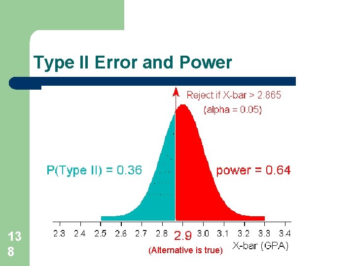
Alternative Decision Rule l l 13 5 “Reject if p-value 0. 05” is equivalent to “reject if the sample average, X-bar, is larger than 2. 865” X-bar > 2. 865 is called “rejection region. ”

Minimize chance of Type I error. . . l l 13 6 … by making significance level small. Common values are = 0. 01, 0. 05, or 0. 10. “How small” depends on seriousness of Type I error. Decision is not a statistical one but a practical one (set alpha small for safety analysis, larger for traffic congestion, say)

Type II Error and Power l l 13 7 “Power” of a test is the probability of rejecting null when alternative is true. “Power” = 1 - P(Type II error) To minimize the P(Type II error), we equivalently want to maximize power. But power depends on the value under the alternative hypothesis. . .

Type II Error and Power 13 8 (Alternative is true)

Factors affecting power. . . l l 13 9 Difference between value under the null and the actual value P(Type I error) = Standard deviation Sample size

Strategy for designing a good hypothesis test l l l 14 0 Use pilot study to estimate std. deviation. Specify . Typically 0. 01 to 0. 10. Decide what a meaningful difference would be between the mean in the null and the actual mean. Decide power. Typically 0. 80 to 0. 99. Simple to use software to determine sample size …

How to determine sample size Depends on experiment Basically, use the formulas and let sample size be the factor you want to determine Vary the confidence interval, alpha and beta http: //www. ruf. rice. edu/~lane/stat_sim/conf_inte rval/index. html 14 1

If sample is too small. . . l … the power can be too low to identify even large meaningful differences between the null and alternative values. – – 14 2 Determine sample size in advance of conducting study. Don’t believe the “fail-to-reject-results” of a study based on a small sample.

If sample is really large. . . l … the power can be extremely high for identifying even meaningless differences between the null and alternative values. – – 14 3 In addition to performing hypothesis tests, use a confidence interval to estimate the actual population value. If a study reports a “reject result, ” ask how much different?

The moral of the story as researcher l l 14 4 Always determine how many measurements you need to take in order to have high enough power to achieve your study goals. If you don’t know how to determine sample size, ask a statistical consultant to help you.

Important “Boohoo!” Point l l l 14 5 l Neither decision entails proving the null hypothesis or the alternative hypothesis. We merely state there is enough evidence to behave one way or the other. This is also always true in statistics! No matter what decision we make, there is always a chance we made an error. Boohoo!

Comparing the Means of Two Dependent Populations The Paired T-test …. 14 6

Assumptions: 2 -Sample T-Test l l l 14 7 Data in each group follow a normal distribution. For pooled test, the variances for each group are equal. The samples are independent. That is, who is in the second sample doesn’t depend on who is in the first sample (and vice versa).

What happens if samples aren’t independent? That is, they are “dependent” or “correlated”? 14 8

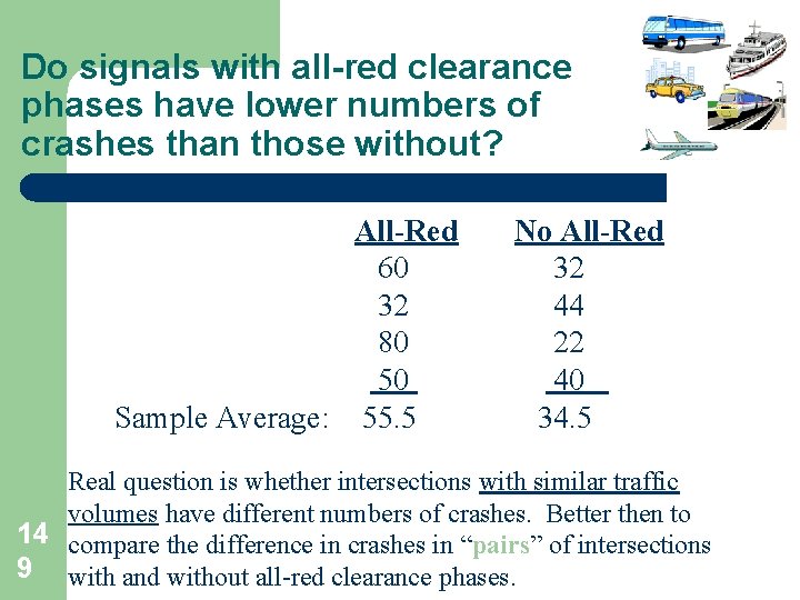
Do signals with all-red clearance phases have lower numbers of crashes than those without? All-Red 60 32 80 50 Sample Average: 55. 5 No All-Red 32 44 22 40 34. 5 Real question is whether intersections with similar traffic volumes have different numbers of crashes. Better then to 14 compare the difference in crashes in “pairs” of intersections 9 with and without all-red clearance phases.

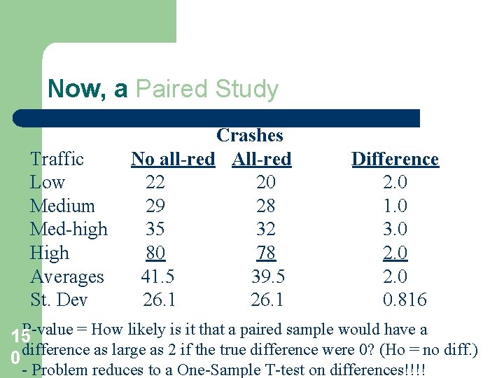
Now, a Paired Study Traffic Low Medium Med-high High Averages St. Dev Crashes No all-red All-red 22 20 29 28 35 32 80 78 41. 5 39. 5 26. 1 Difference 2. 0 1. 0 3. 0 2. 0 0. 816 P-value = How likely is it that a paired sample would have a 15 difference as large as 2 if the true difference were 0? (Ho = no diff. ) 0 - Problem reduces to a One-Sample T-test on differences!!!!

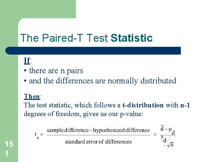
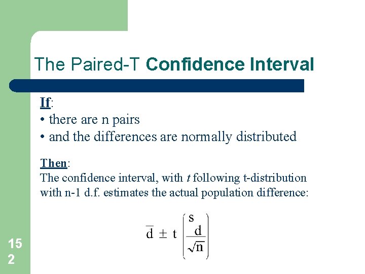
The Paired-T Test Statistic If: • there are n pairs • and the differences are normally distributed Then: The test statistic, which follows a t-distribution with n-1 degrees of freedom, gives us our p-value: 15 1

The Paired-T Confidence Interval If: • there are n pairs • and the differences are normally distributed Then: The confidence interval, with t following t-distribution with n-1 d. f. estimates the actual population difference: 15 2

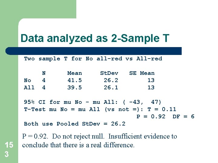
Data analyzed as 2 -Sample T Two sample T for No all-red vs All-red No All N 4 4 Mean 41. 5 39. 5 St. Dev 26. 2 26. 1 SE Mean 13 13 95% CI for mu No - mu All: ( -43, 47) T-Test mu No = mu All (vs not =): T = 0. 11 P = 0. 92 DF = 6 Both use Pooled St. Dev = 26. 2 15 3 P = 0. 92. Do not reject null. Insufficient evidence to conclude that there is a real difference.

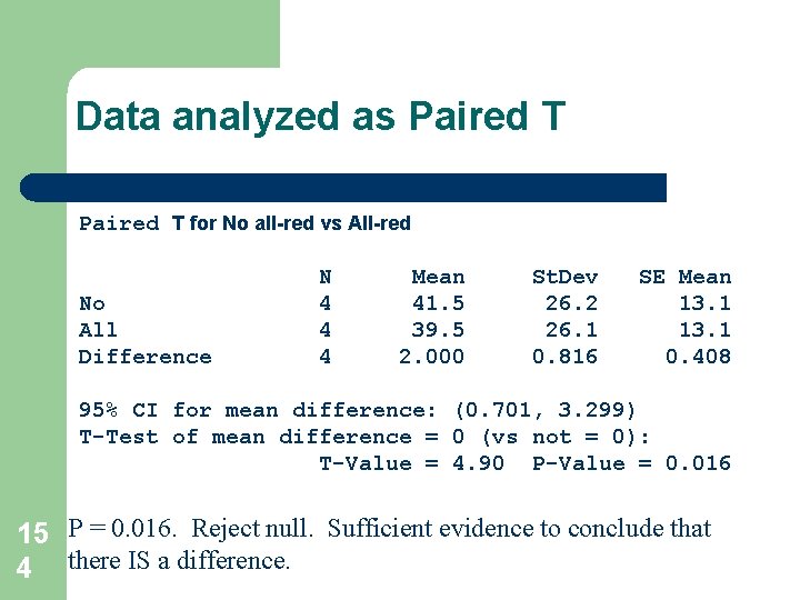
Data analyzed as Paired T for No all-red vs All-red No All Difference N 4 4 4 Mean 41. 5 39. 5 2. 000 St. Dev 26. 2 26. 1 0. 816 SE Mean 13. 1 0. 408 95% CI for mean difference: (0. 701, 3. 299) T-Test of mean difference = 0 (vs not = 0): T-Value = 4. 90 P-Value = 0. 016 15 P = 0. 016. Reject null. Sufficient evidence to conclude that 4 there IS a difference.

What happened? l l l 15 5 P-value from two-sample t-test is just plain wrong. (Assumptions not met. ) We removed or “blocked out” the extra variability in the data due to differences in traffic, thereby focusing directly on the differences in crashes. The paired t-test is more “powerful” because the paired design reduces the variability in the data.

Ways Pairing Can Occur l l l 15 6 When subjects in one group are “matched” with a similar subject in the second group. When subjects serve as their own control by receiving both of two different treatments. When, in “before and after” studies, the same subjects are measured twice.

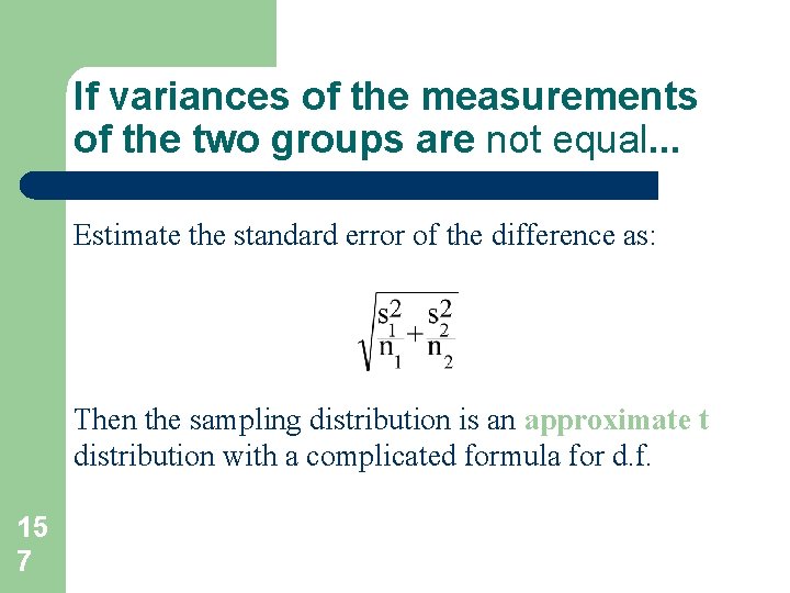
If variances of the measurements of the two groups are not equal. . . Estimate the standard error of the difference as: Then the sampling distribution is an approximate t distribution with a complicated formula for d. f. 15 7

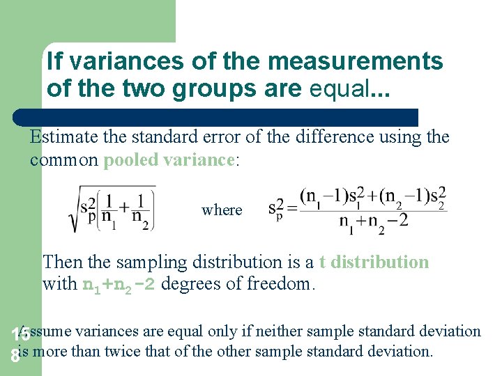
If variances of the measurements of the two groups are equal. . . Estimate the standard error of the difference using the common pooled variance: where Then the sampling distribution is a t distribution with n 1+n 2 -2 degrees of freedom. Assume variances are equal only if neither sample standard deviation 15 8 is more than twice that of the other sample standard deviation.

Assumptions for correct P-values l l l 15 9 Data in each group follow a normal distribution. If use pooled t-test, the variances for each group are equal. The samples are independent. That is, who is in the second sample doesn’t depend on who is in the first sample (and vice versa).

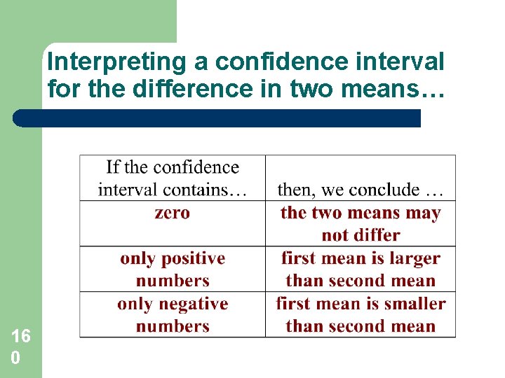
Interpreting a confidence interval for the difference in two means… 16 0

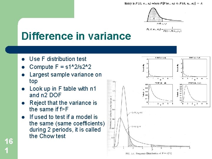
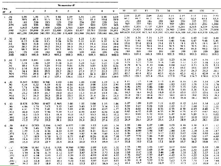
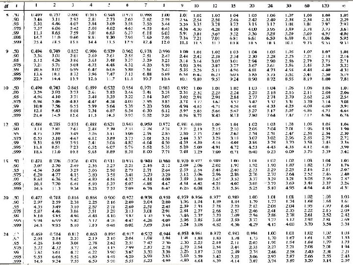
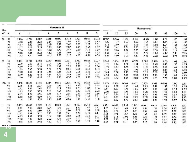
Difference in variance l l l 16 1 Use F distribution test Compute F = s 1^2/s 2^2 Largest sample variance on top Look up in F table with n 1 and n 2 DOF Reject that the variance is the same if f>F If used to test if a model is the same (same coefficients) during 2 periods, it is called the Chow test

16 2

16 3

16 4

Experiments and pitfalls l Types of safety experiments – Before and after tests – Cross sectional tests l Control sample l Modified sample l Similar or the same condition must take place for both samples 16 5

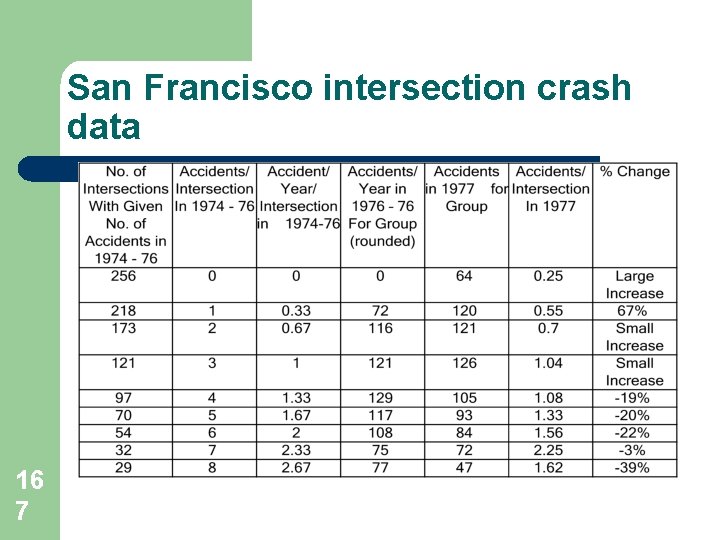
Regression to the mean l This problem plagues before and after tests – Before and after tests require less data and therefore are more popular l Because safety improvements are driven abnormally high crash rates, crash rates are likely to go down whether or not an improvement is made. 16 6

San Francisco intersection crash data 16 7

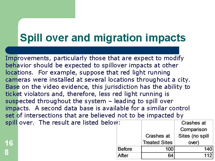
Spill over and migration impacts Improvements, particularly those that are expect to modify behavior should be expected to spillover impacts at other locations. For example, suppose that red light running cameras were installed at several locations throughout a city. Base on the video evidence, this jurisdiction has the ability to ticket violators and, therefore, less red light running is suspected throughout the system – leading to spill over impacts. A second data base is available for a similar control set of intersections that are believed not to be impacted by spill over. The result are listed below: 16 8

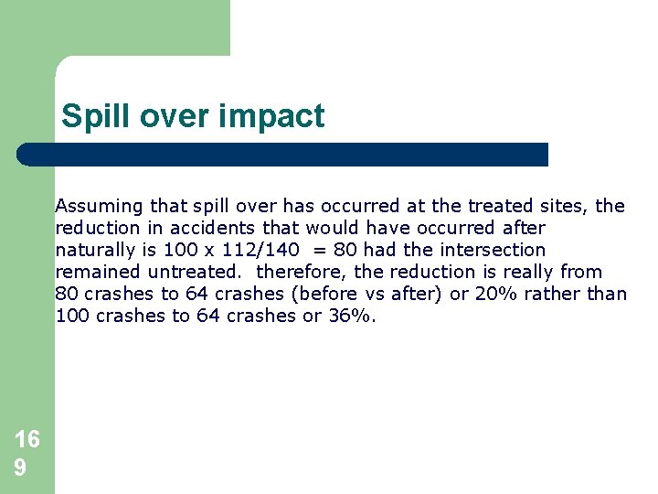
Spill over impact Assuming that spill over has occurred at the treated sites, the reduction in accidents that would have occurred after naturally is 100 x 112/140 = 80 had the intersection remained untreated. therefore, the reduction is really from 80 crashes to 64 crashes (before vs after) or 20% rather than 100 crashes to 64 crashes or 36%. 16 9

Spurious correlations 17 0 During the 1980 s and early 1990 s the Japanese economy was growing at a much greater rate than the U. S. economy. A professor on loan to the federal reserved wrote a paper on the Japanese economy and correlated the growth in the rate of Japanese economy and their investment in transportation infrastructure and found a strong correlation. At the same time, the U. S. invests a much lower percentage of GDP in infrastructure and our GNP was growing at a much lower rate. The resulting conclusion was that if we wanted to grow the economy we would invest like the Japanese in public infrastructure. The Association of Road and Transportation Builders of America (ARTBA) loved his findings and at the 1992 annual meeting of the TRB the economist from Bates college professor won an award. In 1992 the Japanese economy when in the tank, the U. S. economy started its longest economic boom.

Spurious Correlation Cont. What is going on here? What is the nature of the relationship between transportation investment and economic growth? 17 1