WalkSAT with multivalued variables CSE 592 Said AbouHallawa

Walk-SAT with multi-valued variables CSE 592 Said Abou-Hallawa

Outline A quick review of Satisfiability-Problem and Walk-SAT algorithm n Multi-valued variables problem n Problem description language n Problem Data structures n Measurements n

Satisfiability-Problem n n Input: A set of propositional clauses given in conjunctive normal form (CNF) Target: Find an assignment that satisfies all the clauses (if such an assignment exists) Local searches like Walk-Sat have been successfully used for finding satisfying assignments The crucial differences among the local search algorithms are how to choose a variable to be flipped and how to escape from local minima.

Walk-SAT Algorithm Procedure Walk-SAT(P) for i 1 to MAX-TRIES T a randomly generated truth assignment for j 1 to MAX-CHANGES if T satisfies P then return T C randomly selected clause from clauses that false in P With probability p flip the value of randomly selected variable in C else flip the value of the variable that maximizes the number of stratified clauses end for return "No satisfying assignment found"

Walk-Sat with multi-valued variables n n The domain of Boolean variables is {TRUE, FALSE} With multi-valued variables the domains can have more than two values, for example for color variables their domain can be {RED, GREEN, BLUE} As a result, a clause can looks like the following (V 1==RED || V 2==GREEN) This decreases the number of variables used in the problem but it might increase the number of terms per clause

Problem description language n n To state a problem easily and clearly a context free grammar is used. The types of the variables are defined with their domain. type color = {RED, GREEN, BLUE}; Then the variables of a domain are defined var V 1, V 2, V 3, V 4: color; A CNF expression is included representing the problem to be satisfied Graph = (V 1!=RED||V 2!=RED)&& …

Graph Coloring with Boolean variables problem Graph; type BOOLEAN = {T, F}; var var RV 1, GV 1, BV 1, begin V 1 V 2 V 3 V 4 E 12 E 23 E 14 E 34 = = = = = RV 2, GV 2, BV 2, (RV 1 (RV 2 (RV 3 (RV 4 RV 3, RV 4: BOOLEAN; GV 3, GV 4: BOOLEAN; BV 3, BV 4: BOOLEAN; == == (RV 1 (RV 2 (RV 1 (RV 3 T T == == == || || F F F GV 1 GV 2 GV 3 GV 4 || || || == == RV 2 RV 3 RV 4 T T || || BV 1 BV 2 BV 3 BV 4 == == T); T); == == == F) F) F) && && && (GV 1 (GV 2 (GV 1 (GV 3 == == == F F F || || || GV 2 GV 3 GV 4 == == == F) F) F) && && && (BV 1 (BV 2 (BV 1 (BV 3 Graph = V 1 && V 2 && V 3 && V 4 && E 12 && E 23 && E 14 && E 34; end; == == == F F F || || || BV 2 BV 3 BV 4 == == == F); F); F);

Boolean variables versus multi-valued variables n n n The number of Boolean variables is equal to the number of the multi-valued variables times the number of values in their domain All the Boolean variables that represent one multi-valued variable can be FALSE at any stage in Walk-SAT. For example RV 1, GV 1 and BV 1 in the previous graph coloring can all be FALSE. Two or more variables Boolean variables multivalued represent one multi-valued variable can be TRUE at any stage in Walk-Sat. For example RV 1, GV 1, BV 1 in the previous graph coloring can all be TRUE.

Graph Coloring with multi-valued variables problem Graph; type color = {RED, GREEN, BLUE}; var V 1, V 2, V 3, V 4: color; begin E 12 = E 23 = E 14 = E 34 = (V 1 (V 2 (V 1 (V 3 != != != RED BLUE RED BLUE || || || V 2 V 3 V 3 V 4 V 4 != != != RED) && BLUE); RED) && BLUE); (V 1 != GREEN || V 2 != GREEN) && (V 2 != GREEN || V 3 != GREEN) && (V 1 != GREEN || V 4 != GREEN) && (V 3 != GREEN || V 4 != GREEN) && Graph = E 12 && E 23 && E 14 && E 34; end;

Graph Coloring (Continue) problem Graph; type color = {RED, GREEN, BLUE}; var V 1, V 2, V 3, V 4: color; begin Graph = alldiff(V 1, V 2) && alldiff(V 2, V 3) && alldiff(V 1, V 4) && alldiff(V 3, V 4); end;

Example – Quasi-group problem Quasi; type color = {RED, GREEN, BLUE, YELLOW, PINK}; var var var S 11, S 21, S 31, S 41, S 51, begin Rows Cols S 12, S 22, S 32, S 42, S 52, S 13, S 23, S 33, S 43, S 53, S 14, S 24, S 34, S 44, S 54, color; color; = alldiff(S 11, alldiff(S 31, alldiff(S 51, S 12, S 32, S 52, S 13, S 33, S 53, S 14, S 34, S 54, S 15) && alldiff(S 21, S 35) && alldiff(S 41, S 55); S 22, S 42, S 23, S 43, S 24, S 44, S 25) && S 45) && = alldiff(S 11, alldiff(S 13, alldiff(S 15, S 21, S 23, S 25, S 31, S 33, S 35, S 41, S 43, S 45, S 51) && alldiff(S 12, S 53) && alldiff(S 14, S 55); S 22, S 24, S 32, S 34, S 42, S 44, S 52) && S 54) && Quasi = Rows && Cols; end; S 15: S 25: S 35: S 45: S 55:

alldiff’s and Negative Terms n n For each pair of alldiff’s parameters, a clause is generated. Each clause has two negative terms for each possible value of their type. alldiff(V 1, V 2) (V 1 != Red || V 2 != Red) && (V 1 != Green || V 2 != Green) && (V 1 != Blue || V 2 != Blue) n Negative terms are replaced by positive ones of the same literal but for the other possible values of type of the literal except the value in the negative term V 1 != Red V 1 == Green || V 1 == Blue

Problem Data Structure Clauses Table Terms Indices Tables Terms Table Literals Table Types Table V 1==Red Color V 1==Blue V 1 : : : Atoms Table Red Green Blue

Measurements n n The examples I am using are Quasi-group and graph-coloring with large number of variables. All the local search strategies will be compared with Walk-Sat. Walk-SAT is really outperforming all the other local search algorithms with large scale problems The results are measured in terms of time and number of changes done to satisfy a chosen term.

Genetic Optimization of Factory Management Applications of AI, winter 2003 PMP Program Muhammad Arrabi

Intro to the Problem • In a Boeing airplane-parts factory, each manager is assigned a set of parts. • Each part is either manufactured from raw materials, assembled from other parts, or bought from internal or external vendors. • The manager supervises the preparation of a part and manages the vendor relationship. • Managing external vendors takes more time than internal vendors. • Supervising related parts (e. g. same plane) saves time. • Demand on different parts can vary. • Goal: find best division of parts amongst managers to minimize the effort needed and maximize production.

Optimization of Human Activity • Large solution space (~ 75000 parts, ~600 vendors, ~100 managers). • Many fuzzy parameters, should be open for modification (e. g. managing relationships depends on personality) • Can’t use regular mathematical methods. • Suitable for Stochastic Search Methods • My choice: Genetic Algorithms

Using GA for this problem • Start with a random population of lists, each assigns parts to managers. • Use Genetic Algorithms to evolve generations of these lists. • Let the Genetic Engine run until a satisfactory solution is found. • Modify the restrictions and the fitness function, and then repeat the process.

(optional) GA Engine tuning • GA methods used for creating new populations: – – – Copy the best from previous generation Cross the best to create new solutions. Mutate some of the best to create new ones. Shake, which is a small-scale mutation Random new solutions. • After testing 30, 000 values for the methods above, best percentages: Best 15%, Cross 10%, Mutate 5%, Shake 60%, Random 10%.

(optional) Machine Errors • Error: After giving the genetic algorithm a bunch of penalties on the cost of assigning additional vendors, it came back with a best solution that assigns all vendors to very few manager (~4)! • Reason: because assigning all vendors to few managers minimize the number of penalties overall. • Solution: Set a maximum of vendors that can be assigned to one manager.

Evaluation of Searches for Online FPGA Reconfiguration Doug Beal CSE 592 Applications of Artificial Intelligence

Motivation – VLSI Limits • Future VLSI Trends – CMOS hits scaling limits • Nano-scale Alternatives – Chemical self assembly – Nano-imprinting • Implications – Only regular structures – Stochastic process – high error rate

Problems with Nano-scale • Only regular nano-scale circuits possible – Look like FPGAs (Field Programmable Gate Arrays)! • Differences – Many more computational resources – High error rate • Lower MTBF? • Solution – Reconfigure around failures – How?

How to Reconfigure • Sounds like a search – Find new location for computation • Latency restrictions on signals – Reroute signals • Bi-directional breadth-first hardware assisted search – Turn off used wires, send out signals • Implement search model based on FPGA – Each state is a configuration • Goal is configuration that meets all latency restrictions • Heuristic to estimate quality of configuration – After moving to new state, run hardware signal routing

Evaluation

Cost/Benefit Analysis using Bayesian Networks David Beeman CSE 592 Artificial Intelligence Winter 2003

Project Goals • Learn more about Bayesian Networks • Use Inference Diagrams to weigh costs & benefits of stochastic processes

Approach • Choose a game as a sample model • Use Java. Bayes to construct an Inference Diagram • Validate the game’s cost structure or determine the balanced structure • Infer optimal benefit using existing cost structure

Game Description

Game Mechanics

Initial Network

Status/Lessons Learned • Make sure all dependencies are modeled • Minimize number of dependencies per node by adding additional nodes • Automate Java. Bayes input generation • Easy to infer optimal benefit • Still trying to validate Cost Structure

Naïve Bayesian E-Mail Classification Lars Bergstrom 3/6/2003

What’s the problem? • Spam – n. Unsolicited e-mail, often of a commercial nature, sent indiscriminately to multiple mailing lists, individuals, or newsgroups; junk e-mail. Source: The American Heritage® Dictionary of the English Language, Fourth Edition. Copyright © 2000 by Houghton Mifflin Company. Published by Houghton Mifflin Company. All rights reserved. – Any email you get but didn’t want • There’s too much of it! – Average users get a bit – Top-level domain owners and highly visible people get a lot more

What can we do about it? • You can’t really ‘unsubscribe’ or ‘opt-out’ – Added to lists faster than you can remove – They sometimes ignore your request – They sometimes add you to more lists if you reply! • Client-side options – Manual filtering – Automatic filtering

Automatic Filtering Approach • Use something to remove spam from inbox • Errors when filtering – Treating spam as inbox • Sound-alike mails with new words • Not too bad – Treating inbox as spam • Friends forward a silly spam to you • You get a mail that generally looks spam-like • Very, very bad!

Automatic Filtering Manual-Style • Write a whole bunch of rules – Only capture patterns you notice – Take time to author, often more ‘effective’ at removing mail than you want • Feels more efficient, but still takes a lot of time!

Real Automatic Filtering • Smarter options abound – Let some company do it for you • Hint: they don’t do very well right now or this presentation wouldn’t be necessary! • Learning approaches – Serious text classification algorithms – Simple Naïve Bayesian approach • Many have subtle ‘tweaks’

Naïve Bayes • What’s theory? – This is for those who slept through that lecture… • First, learn a bunch of data from some buckets – Probability(word) = (word count + 1) / (vocabulary + total corpus word count) • Then, classify individual emails – Probability(in-corpus, email-words) = Probability(in-corpus) * Apply(*, Map(Probability, email-words))

Analysis (1) • Okay, so how well does it work? – Roughly, 99. 5% accurate on repeated “learn on a random 90%, test on the rest” runs • How did you evaluate this, anyways? – Scheme 48 • Sub-optimal numeric performance • But it handles unboundedly large numbers! – ~2000 spam emails – ~200 inbox emails

Analysis (2) • What are the not-so-useful hacks people tried? – Trying to normalize word forms (Pantel, Spam. Cop) – In general, training on small corpus (Horvitz et al. , Androutsopoulos et al. , several other works) • What are the good hacks? – Just looking at the N most-significant words (Graham, Better Bayesian Filtering) – Word pairs, repetition of URLs (Burton, Spam. Probe)

What’s next? • Other hacks that might prove useful – Sound-alike detection • For the new generation of spam! • Maybe a different weighting for unseen words – Requires a really big corpus phonics! • Or is this already good enough? – Folks agree 99. 7% is about the limit (Burton, Spam. Probe)

Questions?

Robocode “. . . an intelligent creature in a virtual environment. . . ”

What is Robocode? • • • A toolkit for building virtual tank robots An environment for battles of 2 or more tanks Includes a Java applet and API extension Originally created as means to learn Java Seems to have a small, enthusiastic following – Lots of sample robot code available – You can download other people’s tanks to battle against – Occasional group battles referred to as melees • It is kind of fun!

Background • Tank robots begin battle with 100 energy units • You shoot at enemy tanks with “energy” bullets – Shooting costs 0. 1 to 3 energy units (selectable) – If you hit the other tank you get 3*energy back – If you get hit, you lose 4*energy • Battle lost when your energy is depleted

Learnable environment? • Provides a basis for reinforcement learning – Cost for each shot (lose 1 x energy of bullet) – Reward for a hit (gain 3 x energy of bullet) – You lose the battle when your energy is gone • Suggests a learning-enabled robot can gain an edge by shooting only when expected gain exceeds expected cost – e. g. P(hit) >33%

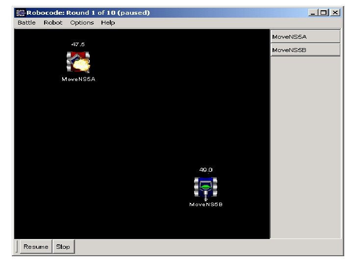
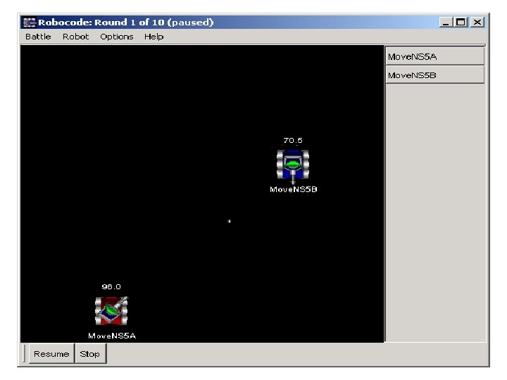
My simplified problem • 2 tanks repeatedly move up/down at a specific X coordinate – their “patrol line” • Stop often to look for enemy tank, shoot – Have to lead a moving target about 5 degrees • Range to enemy is divided into 8 bins; these form input to learning model • Model learns whether the shot is worth taking

Robocode • What does the hit/miss probability look like depending on target range? – Ran a series of 500 battles – Over 10, 000 shots fired • Counted hits and misses by range bin • Data suggests learning can help avoid misses

Robocode

Robocode • Learning models can exploit this knowledge • One approach is a simple perceptron – Boolean inputs, one for each distance zone – Weight for given zone is adjusted depending on whether a shot hit or missed • Lowers weight if we miss (less likely to shoot) • Increases weight if we hit (more likely to shoot) • What does this model look like?

Robocode

A Problem? ? • Small probability that a long sequence of misses could drive the weight below the ‘shoot’ threshold for a zone with overall high expected return for shooting – If that happens, weight will never return to above threshold – Slower learning rate may not be sufficient – Happens because we get negative reinforcement if we shoot and miss; but no feedback when we don’t shoot but would have hit the target if shot was taken • Solution: randomly shoot sometimes even if Perceptron model would suggest not shooting

Improved Perceptron

A better model? • 2 layer neural network • Inputs: Range, Bearing, Location • 4 Outputs: lead on target (3, 6, or 9 degrees) or don’t shoot • Weighting adjusted by back propagation • I may try it and compare to Perceptron • Could look like this:

Two- layer Neural Network Model

Re-implementation of SEER, a Sequence Extrapolating Robot By Jason Chalecki Based on a paper by D. W. Hagelbarger

The Game n n n Each player has a coin. They each decide which side to expose and, at the same time, show each other. If both shown sides are different, the first player wins. If they are the same, the second player wins. A generally safe strategy is to simply choose randomly with equal probability. This can also be played in terms of + and – or 1 and 0 instead of heads and tails.

A Little History n n n Around 1955, D. W. Hagelbarger posited that people don’t play completely randomly and that short periodic sequences emerge. He designed a machine that would detect these sequences, and should be able to win more than 50% on average. Achieved limited success: out of 9, 795 trials with visitors and employees at Bell Labs, it won 5, 218 times and lost 4, 577 times.

Basic Strategy n The machine will recognize four simple periodic sequences q q n ++++… ----… +-+-+-… ++--… While it is still trying to recognize a sequence or if it is losing, it will play randomly.

Implementation of the Strategy (1) n n Since everything is symmetric to + and -, the machine keeps track of plays in terms of same (S) or different (D) play compared to the previous. Machine keeps track of: q q q Whether it won the previous round. Whether it won two rounds ago. Whether it played S or D last round.

Implementation of the Strategy (2) n For each combination (e. g. WSW, WDL LDL), the machine maintains some sub-state: q q q Whether it won the previous round in this sub-state when it followed the recommendation or played randomly. Whether it won two rounds ago in this sub-state when it followed the recommendation or played randomly. A counter keeping track of whether it should have played S or D the last round. If S, 1 is added. If D, 1 is subtracted. The counter is bounded by -3 and 3.

Implementation of the Strategy (3) n n If the counter is positive, the recommended play is S. If it is negative, the recommended play is D. If the machine won the last two rounds in this sub-state, it follows its recommendation. If it won one of the last two rounds in this substate, it follows the recommendation with 3 : 1 odds. If it lost the last two rounds in this sub-state, it plays randomly.

Internals of Recognized Sequences n n n + + and - - SSSS + - DDDD + + - - DSDS SSSS WSW: play S (ctr > 0) DDDD WDW: play D (ctr < 0) DSDS WSW: play D (ctr < 0); WDW: play S (ctr > 0)

Some Weaknesses n n There are some strategies for beating the machine, but they are fairly complex as the opponent needs to keep track of the state the machine is in. For the first several rounds (~10 - 20), the machine basically plays randomly as it tries to learn the sequences.

Questions?

Predictive Text Entry for Traditional Keyboards • Reduce number of keystrokes required for natural language text entry. • Focus on new application of existing methods, rather than exploring new methods.

Inspiration • PTE for small devices is an active area of research. • Specialized PTE applications for desktop machines exist in code editors, accessibility aids, & assisted manual translation app. • PTE not widely used for keyboard-based NL text entry.

Goal IME-like tool that works with other apps.

Smoothing Pest(wi|wi-1) = λPBG(wi|wi-1) + (1 - λ)PUG(wi) Important to separate training & evaluation data (otherwise optimal λ = 1).

Mind Reader: An Improvement of the Original SEER Design Michael D. Helander

SEER • A SEquence Extrapolating Robot, D. Hagelbarger • Built in hardware • Plays a simple matching game with an opponent • Machine wins if its guess matches the opponent and the player wins if the guesses are different • Won approximately 53. 27% of 9795 trials against visitors and employees at Bell Labs in the 1950’s

The Original SEER Strategy • Assumes the play of people will not be random • Tracks the state of play with the following info – whether it won or lost the last play – whether it played the same or different the last time – whether it won or lost the play before last • For each of the eight states it keeps track of – should the machine play the same or different? – has the machine been winning in this state?

The SEER Rules of Play • The machine looks at the information for its state • A counter [-3, +3] tracks whether the machine should play the same (+) or different (-) • If the machine has lost the last two in this state it plays randomly with equal likelihood • If the machine has won once in the last two it has 3: 1 odds it will follow the counter’s instructions • If the machine has won the last two in this state it follows the recommendations of the counter

My Version: Mind Reader • Utilizes an order 4 decision tree of depth 5 • A collection of predictors sharing the same decision tree with each looking at a different depth (i. e. a varying amount of player history) • A simplistic prediction algorithm within each predictor that assumes player will repeat their play • A selector for choosing the ultimate prediction for the program from among the options produced by the predictors

Mind Reader Operation Win Dif True Diff e am True Same ss. S W Lo Lo in Sa me f Player Won Same or Diff False Diff ss. D iff False Same

An Analysis of the Initial Version • Level 1 predictor performs poorly (the final value for the accuracy score was typically around -10) • Additional selector algorithms should be looked at beyond the original implementation – S 0: Majority, breaking ties with random play (original) – S 1: Majority, breaking ties with highest accuracy score – S 2: Predictor utilizing the most history – S 3: Predictor with the highest accuracy score

Will vs. the Mind Reader • Will’s guesses were in a pattern of heads and tails – 1 heads, 2 tails, 3 heads, 4 tails, 5 heads, etc. • This high score shows the program’s ability to fairly quickly recognize patterns and adjust its picks accordingly

Remaining Work • Look at adding one more layer above the selectors and keep track of accuracy measures for the individual selector algorithms • See how well the machine plays when using the selector with the highest accuracy score instead of having to pick one that is used throughout the run • Look at tailoring the accuracy scores so that only recent history is taken into account and not the overall accuracy for the entire game • Modify predictor algorithm to take into account current trends for that level of play

Questions?

SEER: SEquence Extrapolating Robot Chan Im CSE 592 - Artificial Intelligence Winter 2003

Overview of SEER n n A machine developed by David W. Hagelbarger at Bell Labs in 1955. Plays a game called “Matching Pennies”. Player B tries to match the coin flip of Player A u 50% probability of success in random play u n Designed to show that machines can adjust to changing environments. No need to redesign the system u Applications in telephony - i. e. call routing u

SEER’s Game Strategy n Human behavior in “Matching Pennies” are not totally random. u n Determine a pattern in the sequence of the human opponent’s play. u n n Data model is unknown 4 Simple periodic sequences u n Emotion, cheating, or a “system” affects a person’s game playing behavior. ++++, ----, +-+-+-, ++--++ Challenge: Match > 50% 9795 plays: won 5218, lost 4577 => 53%

SEER Implementation n n Initially, machine plays randomly until a pattern is found. Coin matching based on 3 “state of play” Did it win or lose last play? u Did it win or lose the play before last? u Did it play same or different? u n Leads to 8 possible states with 2 data: a) Play same or different to win? b) Has it been winning in this state?

SEER Implementation n n Take action based on data at each state. If it has lost the last 2 times in this state: u n If won one and lost one in this state: u n Play randomly Play same with 3 -to-1 odds on same side If won last 2 times in this state: u Always play same side in state data (a)

How To Beat SEER n Figure out what the machine is going to play. u n Need to keep track of the memory content for each state during each game. Change play pattern after establishing a pattern recognized by the machine. u Difficult to do for large number of games.

AI Techniques n SEER uses probability theory based on past data to determine what present actions to take. u n Otherwise, it plays randomly. Can apply simple decision network Transition from state to state based on action from prior state. u Other states have low utility u

TD-Gammon in C# Richard Katz & Lin Huang

Neural Net Output: Predicted Probability of Winning

198 Encoded Input Units • 24 Locations with 8 Units Each: - 1 or more White (0 | 1) - 2 or more White (0 | 1) - 3 or more White (0 | 1) - 4 or more White (n-3)/2 - 1 or more Blue (0 | 1) - 2 or more Blue (0 | 1) - 3 or more Blue (0 | 1) - 4 or more Blue (n-3)/2 • Bar Locations: - White (n/2) • Pieces Off Board: - White (n/15) • Turn to Move: - White (0 | 1) - Blue (n/2) - Blue (n/15) - Blue (0 | 1)

Neural Net Training Rules • Temporal difference weight change formula: t wt+1 - wt = a (Yt+1 - Yt ) S l k=1 t -k Ñ w Yk • Gradient for hidden-to-output weights: Yo (1 - Yo ) Yh • Gradient for input-to-hidden weights: Yo (1 - Yo ) wh, o Yh (1 - Yh ) xi • Eligibility traces of decaying contributions: e t = l e t -1 + Ñ w Y t

Results of TD-Learning

TD-Gammon in C# Experiments: 1 M Training; Unit Encoding; a l; Hidden® 80

Crossword Puzzle Generation By Alia Nabawy

The Problem l Given: – – l Dictionary of words. Crossword puzzle with a certain layout. Find – Layout of words from dictionary to fit into the puzzle.

How to solve problem ? l For puzzles greater than 4 x 4 brute-force depth first search is impractical. l Need to use some heuristics

Common Heuristics used l l Cheapest-first Connectivity Lookahead Intelligent instantiation

Cheapest-first l l Fill in words that have the smallest candidate lists. These words are typically: – – l Longer words. Partially-filled words. Justification: Solve hard words first, more likely later words will have solutions at all.

Connectivity l l l Used for reducing backtracking. Backtrack NOT to previously completed word but to the oldest word intersecting current failing word. No need to waste steps regenerating words that are not the cause of problem.

Connectivity Example: Order of filling: t a b l e a l a r m (1) table (2) alarm (3) calls (4) lr… (2) Don’t backtrack to calls but to table and regenerate all words again. c a l l s

Intelligent Instantiation l l l Why just pick the first candidate word ? This technique treats the first k candidate words fairly. For each candidate wi compute number of possibilities for each intersecting word and then compute product of all these values. Choose wi that maximizes this value. Idea is to choose a candidate word that maximizes the number of possibilities for later intersecting words.

Lookahead l l l Simple check: Before a word is filled, candidate lists for all intersecting words are checked. If any of the lists are empty discard the word and look for another candidate. Can be used in conjunction with any of the other heuristics.

Scheduler Arwen Pond CSE 592

FASTPASS® Can have only one pass at a time Must physically go to the ride to get that pass Scheduler Schedule as many rides as you want Go to any ride to schedule

Annealing Options Starting Temperature Dampening Number of times without Changes

Sample Schedule Ride Time Ride Duration Walking Time Autopia 8: 00 am 0 26 Big Thunder Mountain 8: 30 am 4 16 Splash Mountain 9: 00 am 9 6 Haunted Mansion 9: 30 am 8 6 Pirates of the Caribbean 9: 45 am 16 6 Indiana Jones 10: 15 am 5 18 Star Tours 10: 45 am 4 4 Space Mountain 11: 00 am 3 18 Autopia 11: 30 am 8 28 Roger Rabbit's Car Toon Spin 12: 15 pm 3 Total Time: 255 minutes Total Walking Time 128

Diamond = 10 times without change Circle = 30 times without change Triangle = 70 times without change Square = 100 times without change

function Compute. Schedule() { do { temperature = temperature/n. Dampen. Factor; Change. Node(); }while (n. Times. Without. Change < n. Goal. Times. Without. Change+1); } function Change. Node() { //Choose an invalid node at random and change either the order <Choose 2 random different numbers between 0 and the number of rides-1> //switch the order <Switch nodes Rides[n] and Rides[n 2]> //Compare the total time of the schedule to the previous total time if (n. New. Current > n. Current. Total. Time) { //If this order isn't better then there is a percent //chance that we will keep it anyway. This chance is based //on the current temperature. var chance=(99*Math. random()); if (chance < temperature ) { //We keep the current config even though it is worse and reset //the number of times without change n. Times. Without. Change=0; } else { //We go back to the better config <Switch the order of Ride[n] and ride[n 2] back to original> n. Times. Without. Change++; } } else { //Keep current configuration and reset the number of times without change n. Times. Without. Change = 0; } }

Future Enhancements • Bayesian net that figures the probability of a person showing up on time given variables such as current temperature, number of people in the park, number of people from out of state etc. • Add location information so you can find other people in your party. • Be able to change the schedule throughout the day

Applying Naïve Bayes to Classifying Junk Email CSE 592 Final Project Alfred L. Schumer Winter 2003

Overview n n Implemented as Win 32 command line utility that classifies email messages saved to disk as text files. Examines factors using a local search algorithm that yield the best classification results. Implements a method by which false classifications are reduced via dynamic pruning. Combines local search and pruning into global search function that seeks optimum classification score.

General Approach n n Analyze two corpuses of valid and junk emails and build a Bayesian network of junk word probabilities. Classify two other known corpuses of randomly selected sample test files and give an overall score. Compute optimum parameters yielding the highest success rate in classifying valid and junk emails. Identify and remove words in messages falsely classified having greatest contribution to errors.

Implementation n n Classification, searching and pruning can be combined in any order, any number of times. Supports other features such as condensing and parsing that are typically run once. Other utilities written that renumber files for ease of identification and randomly swap files for sampling. Results sent to the standard output and captured via command line redirection.

Email Corpuses n n Required corpus of junk and valid emails, from which a subset were extracted as test samples. Compiled ~3000 junk and ~1800 valid messages, and randomly extracted 200 each for test samples. Each class placed in unique subdirectory, hard-coded into program comprising working directories. Directories named Junk Corpus, Valid Corpus, Junk Samples and Valid Samples.

Tokenization & Hashing n n Parsed files are tokenized using starting, word and ending tokens resulting in alpha-numeric words possibly hyphenated and possessive. All words over two chars parsed though not used depending on the minimum word length specified. n Did not have time to investigate word stemming. n Word tokens are hashed according to Horner’s Rule. n Floating point closed hash tables prime in size.

Condensing n n n Corpus and sample files have the possibility of being parsed and classified frequently. Condense added to optimize file contents. Reduces files in working directories to sorted, unique word lists. Only needs to be run the first time or when files are added to the working directories. Significantly improves processing time of commands.

Parsing n n Tokenizes corpus files, counts word frequencies, and calculates junk probability. Words that appear in one corpus but not other are assigned probabilities of 1% or 99%. Otherwise, the probability is calculated as: P = (Junk/n. Junk)/((Junk/n. Junk)+(Valid/n. Valid)) Should be called before other functions each time the corpuses change, or pruning is performed.

Classification n n Heuristic for measuring success is percentage of messages falsely (or correctly) classified. Different weighted costs assigned to false positives and false negatives. Score returned from Classify function that classifies the sample files in the working directories. Classification depends on minimum word size, word count, analysis threshold and junk threshold.

Classification State Space

Pruning n n Recursively classifies junk and valid samples tracking misclassified files. Attempts to remove words contributing most to misclassifications. Groups common, duplicated words from misclassified files and rank orders them by probabilities. Removing the most significant word from statistical base, and then recursively prunes again.

Global Search n n Highest-level command seeks to iteratively search and prune data until global maximum is found. Code trivial building on Prune and Search functions: while (true) { Prune (…) Search (…); if (New Score > Best Score) Best Score = New Score; else break; }

Test Results Test Type Classification Score Time (seconds) Search Only 88. 5% 192. 90 Prune Only 88. 8% 34. 255 Search & Prune 92. 5% 226. 691 Global Search 93. 0% 476. 514

Conclusions n n Most work being done today has to do with inputs as discrete words and applying Bayesian principles. Project shows that searching and pruning (especially as Global Search) significantly improves accuracy of applying Naïve Bayes theory. Results showed improvement in classification scores on the order of 83% to 93%. Corpuses work best when they are from the same email user.

Terrarium Project Winfred Wong CSE 592 Winter 2003

. NET Terrarium Project A multiplayer ecosystem game developed using the. NET Framework Creatures in the Terrarium ecosystem compete for resources Types of Creatures: n n n Plants – feed on Sun light ONLY Herbivores – feed on Plants ONLY Carnivores – feed on Herbivores ONLY Creatures can reproduce, die from old age/disease, get killed in battles. Terrarium official homepage: n http: //www. gotdotnet. com/terrarium/

Actions, States and Events Actions on each turn n Move, Eat, Attack, Defend, Reproduce, nop Creature States n Boolean values Is. Alive, Is. Moving, Is. Eating, … n Numeric values Percent. Energy, Percent. Injured, … Events n Born. Event, Idle. Event, Attack. Event, …

Problem Definition Study the effects of states and actions on a herbivore’s survival in the ecosystem – a classification problem Scope n n n Closed environment – no connection to other network Fixed sets of species – two plant species, one herbivore specie, one carnivore specie No communication among creatures Steps n n n Use prototype herbivore to collect data Use WEKA J 48 classifier to generate decision tree based on the data Deduce interesting rules from decision tree

Data Collection Attributes n n n n Hungry : {‘yes’, ’no’} Has. Plant : {‘yes’, ’no’} Has. Threat : {‘yes’, ’no’} Eat : {‘yes’, ’no’} Move : {‘yes’, ‘no’} Attack : {‘yes’, ‘no’} Defend : {‘yes’, ‘no’} Hungry Has. Plant Has. Threat Eat Move Attack Defend Class yes no no no yes no no Bad no yes no no no Good yes yes no no Bad yes no no yes Bad no yes no no no yes Bad no no yes Good Class n n Condition of the herbivore in next turn : {‘good’, ’bad’} Use a combination of health and threat level Percent. Energy > 30% and ~Has. Threat

Analysis Interesting observations: n Attack and Defend are not factors n ~Hungry ^ Has. Threat ^ Move => Good n ~Hungry ^ Has. Threat ^ ~Move => Bad Is running away the only way to survive when a herbivore meets a carnivore? n In most case, yes. n However, statistics showed a small number of carnivores were killed by herbivores.

Analysis (cont’d)

Analysis (cont’d) Herbivores can defend carnivores in some cases, why doesn’t it show up in the decision tree? Missing attributes n Need more data to show this fact n Add Healthy : {‘yes’, ’no’} -- Percent. Injured < 50% n Add Attacker. Healthy : {‘yes’, ’no’} -- attacker. Percent. Injured < 50% Hungry Has. Plant Has. Threat Eat Move Attack Defend Healthy Attacker Healthy Class yes no no no yes no no Yes ? Bad no yes no no no Yes ? Good yes yes no no No Yes Bad yes no no yes Yes No Good no yes no Yes No Good no no yes no No yes Yes Bad

Demo

A Study of Iterated Prisoner’s Dilemma CSE 592 Class Project. By Man Xiong

A Formal Model for Cooperation in Game Theory Cooperate Defect R=3 S=0 Cooperate R=3 T=5 P=1 Defect S=0 P=1 n n T>R>P>S 2 R>T+S

Strategies in Different Game scenarios n Iterated: n n Tit-For-Tat With chaos: n n Tit-For-2 -Tat Generous Tit-For-Tat (p): p: cooperates 1 -p: tit for tat n Pavlov (n): P <- 1/n p += 1/n if the other agent cooperates P: cooperates; 1 -p: defects

Implementation and Simulation n n Implemented in C++ for fast simulation Iteration Tournament: two agents per strategy Chaos Evolution

Self-tuning GTFT and Pavlov n n At the very beginning, the parameter for each agent obey normal distribution For every generation, the value of the parameter of most successful agents is used as the median value for distribution

Balanced 3 SAT Problems and Instance Generator CSE 592 Artificial Intelligence University of Washington Dajun Xu

Introduction Hard satisfiable 3 SAT problems can be used to benchmark and fine tune new algorithms. l How to generate hard 3 SAT formula has always been a challenging topic. l Problems become hard at critical point l Claimed that problems even harder when the “signs” are balanced for each variable l

Project Goals l Create a generator for this type of 3 SAT formula. l Study the phase transition behavior and look for the critical point if there is one. l Find out if this type of problems is really hard in comparison to the regular random 3 SAT problems

Traditional Approach l Generate a random truth assignment T l Construct a formula with N variables and M random clauses l Throw away any clause that violates T l For 3 SAT hard problems, set M = 4. 25 N

Traditional Approach cont. In principle generate all possible satisfiable formulas with a clause-tovariable ratio of 4. 25 that have T among their solution l Somewhat surprising result is that the sampling of these formulas is far from uniform, biased towards formulas with many assignments, clustered around T and easy for Walksat l

Seeding Approach A “Forced” approach, namely start with a random truth assignment l Use “equivalent literals” as seeds to plant in clauses / sentences l For example, (A, -B, -C) is the equivalent literals to an assignment (1, -1) Generator controls randomness of variables and balance of signs l Easy implementation l Efficient enough to construct some hard problems in comparison to random 3 SAT l

Assumptions Each variable must appear at least once in a sentence, but can be either positive or negative or both l No same variable, regardless of sign, in each clause l For example, (A, -A, B) or (A, A, B) are considered to have same variable l Each clause has exactly three literals, this just for easy implementation.

Assumptions, cont. l No two clauses have exact same constructs, regardless the appearing order For example, (A, B, C) and (C, B, A) are considered to have the exact same constructs l The number of clauses M is not less than the number of variables N We are only interested in generating hard problems. All satisfiable problems are easy for Walksat when M is small.

Generator Details l Generate a random truth assignment of size N. l Generate the equivalent literals of size N from the truth assignment as the seeding literals. l Randomly assign each of equivalent literals exactly once to N of M clauses.

Generator Details, cont. l Fill each of rest clauses with one randomly selected equivalent literals Since each clause has at least one equivalent literal. The sentence can be guaranteed satisfiable. l From now on, keep track of the number of positive and negative sign for each variable including those from those created in previous steps.

Generator Details, cont. If any variable is not balanced, repeatedly select the variable with negated sign and put it to a randomly selected clause, until this variable balanced. l If all variables are balanced, randomly select one from 2*N literals, regardless equivalent to truth assignment or not, to a randomly selected clause such that l - No same variable - Less than 3 literals - No same clauses exist in the sentence

Searching for Critical Point l l l Basically a binary search Look for point (number of clause) at which Walksat has the max runtime Measure runtime by the median number of flips Sample 100 points in search range each time 15 Sentences for each point 10 runs Walksat for each sentence due to stochastic nature of Walksat

Comparison of Hardness l Generate 1000 sentences for the critical points found by the balanced 3 SAT generator l Load the benchmark sentences downloaded from www. satlib. org l Run both against Walksat and compare results.

Results: 50 Variables l l l Balanced 3 SAT 50 variables 46200 sentences Critical point found at 184 Clause-Variable ratio = 3. 68

Results: 100 Variables l l l Balanced 3 SAT 100 Variables 64800 sentences Critical point found at 355 Clause-Variable ratio = 3. 55

Results: Balanced vs Random 25 50 75 100 125 150 200 Balanced Random Critical Point Clause-Var Ratio 104 184 275 355 429 510 676 4. 16 3. 68 3. 67 3. 55 3. 43 3. 40 3. 38 112 218 324 430 536 642 854 4. 48 4. 36 4. 32 4. 30 4. 29 4. 28 4. 27

Results: Hardness Comparison 50 Balanced Avg Flips 1445. 095 Random Avg Flips 653. 917 100 8031. 563 3656. 377

References Generating Satisfiable Problem Instances Achlioptas, Kautz (2000) l Balance and Filtering in Structured Satisfiable Problems - Kautz, Ruan, Achlioptas, et al(2001) l Experimental Results on the Crossover point in Random 3 SAT - Crawford (1996) l Using CSP Look-Back Techniques to Solve Exceptionally Hard SAT Instance – Bayardo, Schrag (1996) l

Robo. Code Wesley Yang Olivia Yang

Introduction of Robo. Code l What it is? It is a programming game which lets you create virtual "Robots, " real Java objects that battle against other robots. l How to play? – 2 D movement and fire – Rules

How to predicate movement? l 3 possible methods – Move straight – Acceleration – Curve l Using Bayesian learning

When to fire? l Factors to be considered – Correctness of predication – Bullet hit/missing ratio – Distance to object – Energy status of all opponents

Demo