W 1 B Outline 1 Maths Appendix 1
W 1 B Outline 1 Maths Appendix 1. 1 growth rates, 1. 2 exponents and logs, 1. 3 elasticity 2 National Accounts 2. 1 -2. 3 historical genesis and war 2. 1 1600’s Mercantilism, Petty and Davenant 2. 2 Bolsheviks and WWI: Input Output Analysis 2. 3 WWII: Keynes, Kuznets and Stone 2. 4 Product vs. Expenditure vs. Income Measures 2. 5 Text on Savings identities 2. 6 Real vs Nominal GDP 2. 6. 1 Chain Method 2. 6. 2 Hedonic Methods & CPI vs. PCE price indices 2. 7 Wellbeing vs GDP (Time Permitting) 1

ECO 306 Home Page http: /www. depaul. edu/~jberdell Select Eco 306 ID: macro PW: theory 2

1. 1 Proportional growth rate 3

1. 1 Percent Growth Rate 4

1. 2 Exponent Notation 5
1. 2 Exponent Notation Cont. 6

Solve me! • Let s=1/5, n=1/20, d=1/20 • sk^(1/2)=(n+d)k • What is k? 7
1. 2 Monthly vs Annual Growth 8
1. 2 Quarterly vs Annual Growth 9
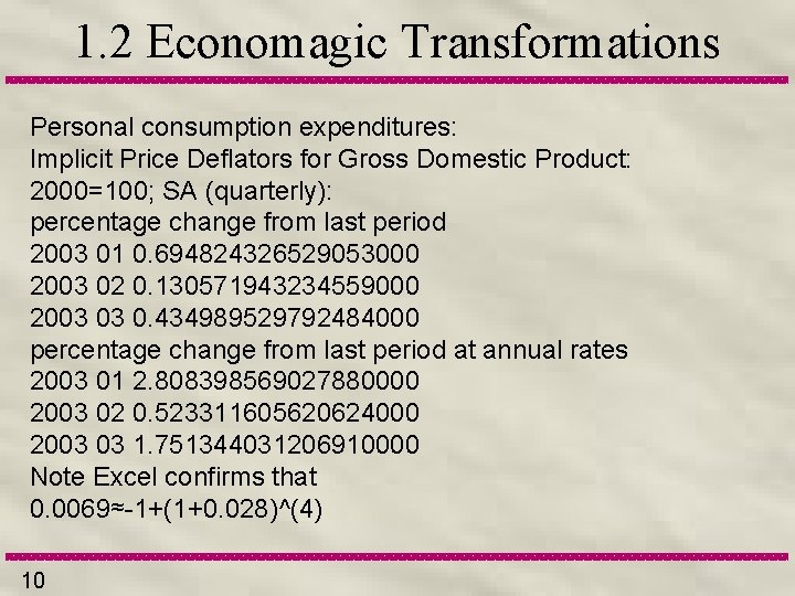
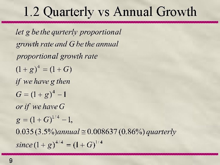
1. 2 Economagic Transformations Personal consumption expenditures: Implicit Price Deflators for Gross Domestic Product: 2000=100; SA (quarterly): percentage change from last period 2003 01 0. 694824326529053000 2003 02 0. 130571943234559000 2003 03 0. 434989529792484000 percentage change from last period at annual rates 2003 01 2. 808398569027880000 2003 02 0. 523311605620624000 2003 03 1. 751344031206910000 Note Excel confirms that 0. 0069≈-1+(1+0. 028)^(4) 10
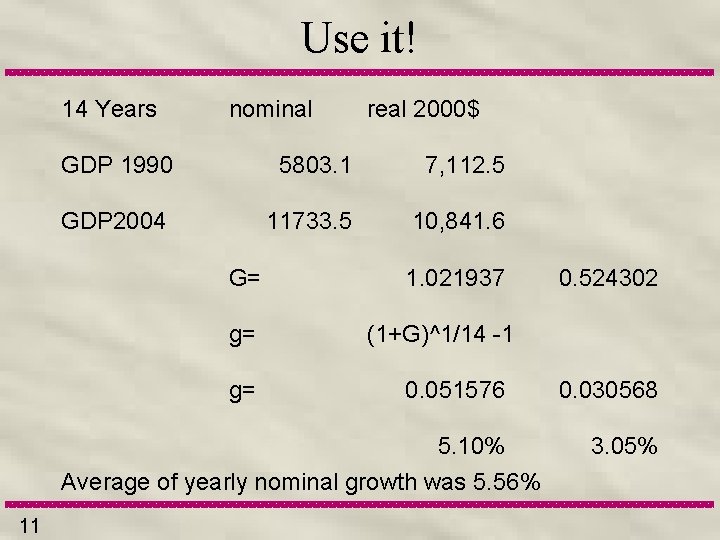
Use it! 14 Years nominal real 2000$ GDP 1990 5803. 1 7, 112. 5 GDP 2004 11733. 5 10, 841. 6 G= g= g= 1. 021937 (1+G)^1/14 -1 0. 051576 5. 10% Average of yearly nominal growth was 5. 56% 11 0. 524302 0. 030568 3. 05%
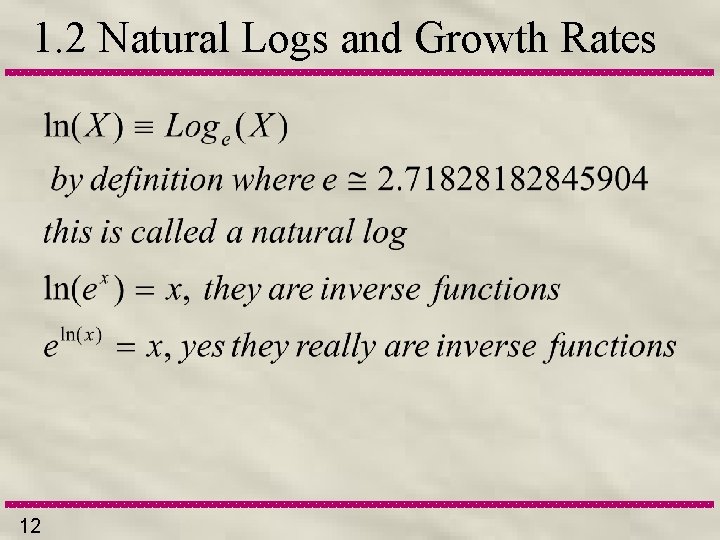
1. 2 Natural Logs and Growth Rates 12
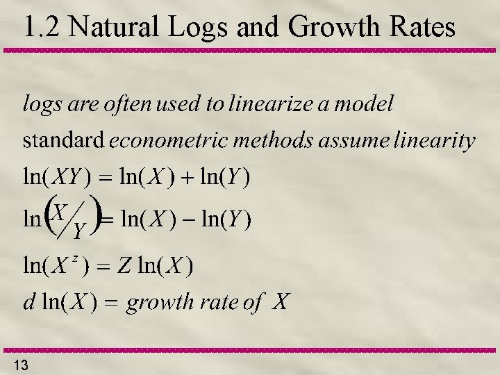
1. 2 Natural Logs and Growth Rates 13
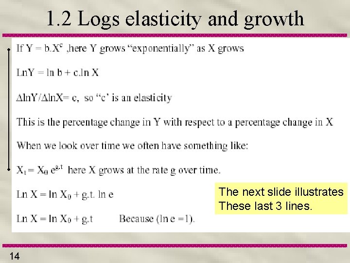
1. 2 Logs elasticity and growth The next slide illustrates These last 3 lines. 14
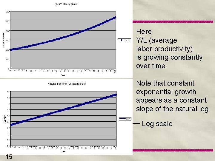
Here Y/L (average labor productivity) is growing constantly over time. Note that constant exponential growth appears as a constant slope of the natural log. Log scale 15
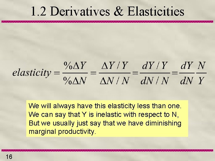
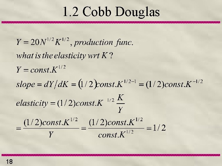
1. 2 Derivatives & Elasticities We will always have this elasticity less than one. We can say that Y is inelastic with respect to N, But we usually just say that we have diminishing marginal productivity. 16
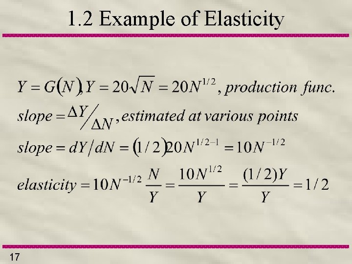
1. 2 Example of Elasticity 17
1. 2 Cobb Douglas 18

• Exponents commonly are elasticities. 19

National income accounts • First attempts to collect information on the whole economy of nation states starts in the mercantilist period. • National Income • National Savings • The Balance of Trade 20
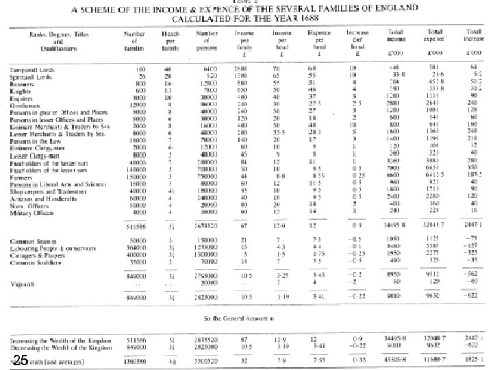
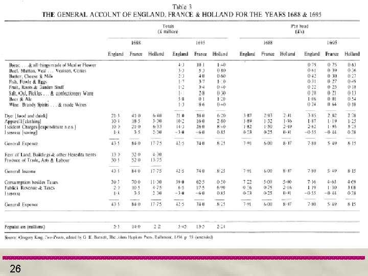
2. 1 Mercantilism Mercantilists How to further power and plenty? Economic growth with greater military might. Growth sometimes regarded as BOT surplus, other times as savings and investment. Petty 1664 and Davenant 1688 were the first attempts to measure savings and growth sources. Source for following slides: http: //www. sjcny. edu/~kaplan/pdf/stone_86. pdf 21
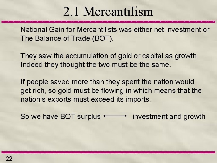
2. 1 Mercantilism National Gain for Mercantilists was either net investment or The Balance of Trade (BOT). They saw the accumulation of gold or capital as growth. Indeed they thought the two must be the same. If people saved more than they spent the nation would get rich, so gold must be flowing in which means that the nation’s exports must exceed its imports. So we have BOT surplus 22 investment and growth
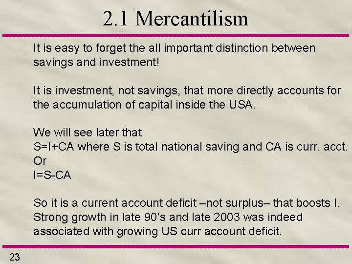
2. 1 Mercantilism It is easy to forget the all important distinction between savings and investment! It is investment, not savings, that more directly accounts for the accumulation of capital inside the USA. We will see later that S=I+CA where S is total national saving and CA is curr. acct. Or I=S-CA So it is a current account deficit –not surplus– that boosts I. Strong growth in late 90’s and late 2003 was indeed associated with growing US curr account deficit. 23
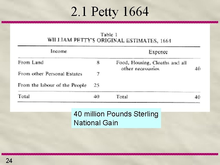
2. 1 Petty 1664 40 million Pounds Sterling National Gain 24
25
26

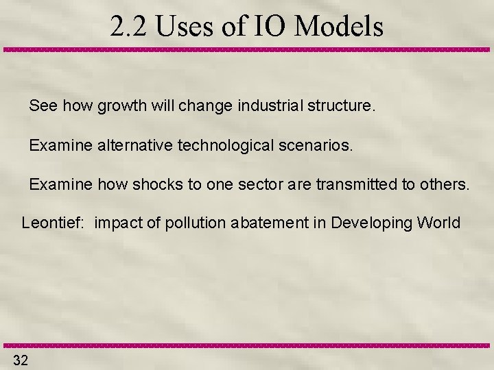
2. 2 Leontief Input Output IO tables show industries are interrelated. Displays the use of each sector’s output by other sectors and by final demanders. 27

2. 2 BEA Make-Use Tables 28
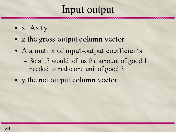
Input output • x=Ax+y • x the gross output column vector • A a matrix of input-output coefficients – So a 1, 3 would tell us the amount of good 1 needed to make one unit of good 3 • y the net output column vector 29
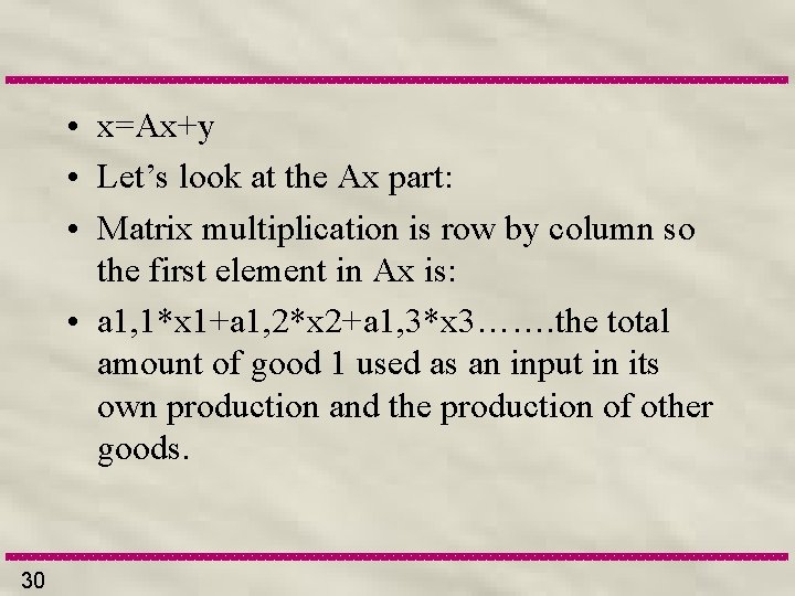
• x=Ax+y • Let’s look at the Ax part: • Matrix multiplication is row by column so the first element in Ax is: • a 1, 1*x 1+a 1, 2*x 2+a 1, 3*x 3……. the total amount of good 1 used as an input in its own production and the production of other goods. 30

2. 2 Link to BEA Use Table The Use of Commodities by Industries before redefinitions BEA Industry Accounts Home Page http: //www. bea. doc. gov/bea/dn 2. htm 31
2. 2 Uses of IO Models See how growth will change industrial structure. Examine alternative technological scenarios. Examine how shocks to one sector are transmitted to others. Leontief: impact of pollution abatement in Developing World 32

2. 3 Simon Kuznets Institutionalist follower of Wesley Mitchell Emphasizes changes in Economic structure and Ideology in process of Modern growth. 1973 Nobel Lecture from the American Economic Review ‘Modern Economic Growth’ http: //www. sjcny. edu/~kaplan/pdf/kuznets_73. pdf 33

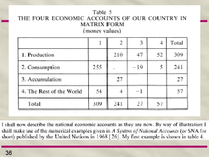
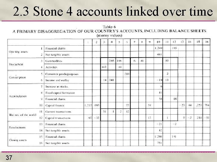
2. 3 Sir John Richard Nicholas Stone, 1913 -1991 First UK national accounts produced during WWII in consultation with Keynes. This formed the basis for UN system. 34

2. 3 Volatility: Keynes was interested in spending and effective demand 35
36
2. 3 Stone 4 accounts linked over time 37
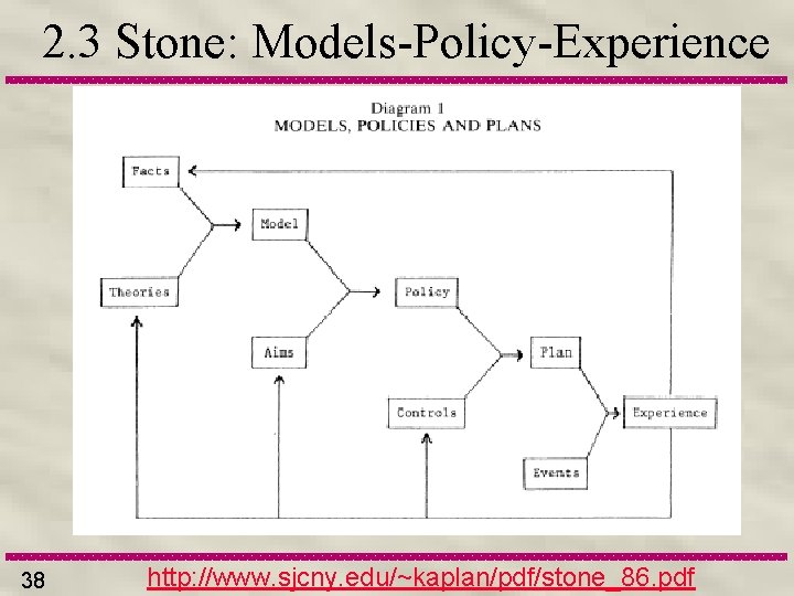
2. 3 Stone: Models-Policy-Experience 38 http: //www. sjcny. edu/~kaplan/pdf/stone_86. pdf

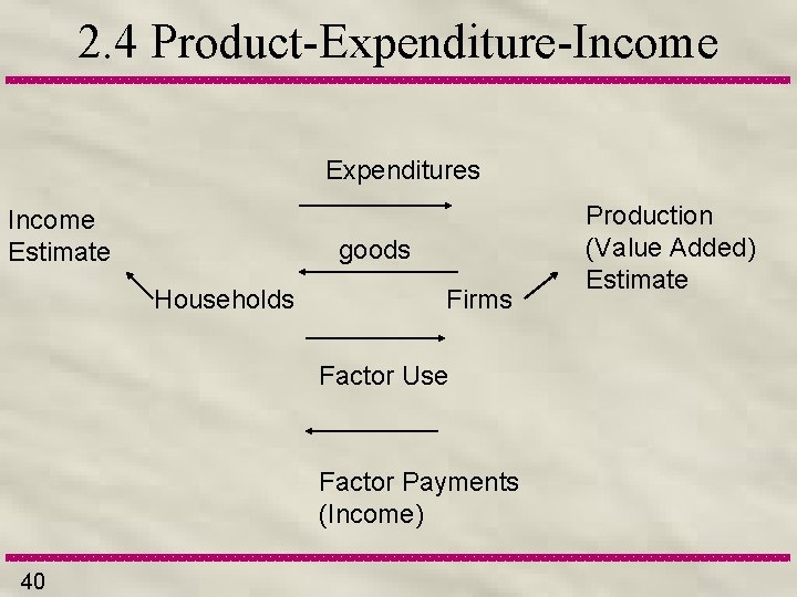
2. 4 Text on GDP A&B suggest that there are 3 different ways to estimate GDP! Expenditure, Product and Income. There is really no difference between expenditure And product in practice. The information for the ostensibly different expenditure and income measurements is not independent. 39
2. 4 Product-Expenditure-Income Expenditures Income Estimate goods Households Firms Factor Use Factor Payments (Income) 40 Production (Value Added) Estimate

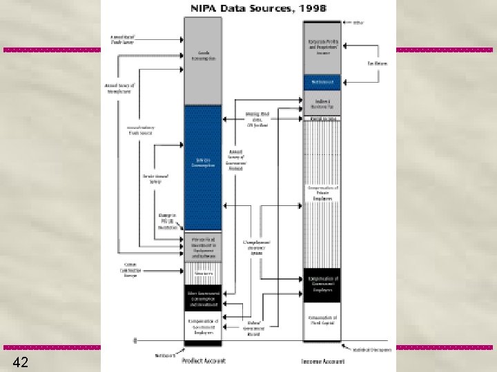
2. 4 Sources for US NIPA Feeding the National Accounts Joseph A. Ritter Review Federal Reserve of St. Louis March/April 2000 http: //research. stlouisfed. org/publications/review/00/03/0003 jr. pdf 41
42

2. 4 A Witch's Brew? John Haltiwanger (1997) described the impression many economists have ofthe NIPA: “This depiction [of the NIPA] causes one to imagine that aggregate statistics emerge from some great black cauldron, mixed together with data from an alphabet soup of surveys (p. 68). ” 43
(2. 4) 3 Tiers of GDP estimates 5 Year bench marks with comprehensive Business surveys: These also form the I/O tables (Housing and other items on separate schedules) Annual Estimates Quarterly Estimates 44

2. 4 Regarding the US NIPA: 1) We do not have independent sources for all items. The same information is used in product and income calculation. 2) Personal consumption of durable goods vs. Business Investment. 3) Government Investment—Not in USA till 1996 text books still sweep it under the rug 4) Education appears as consumption of services for households or as current spending (not investment) for government. 45
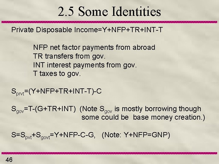
2. 5 Some Identities Private Disposable Income=Y+NFP+TR+INT-T NFP net factor payments from abroad TR transfers from gov. INT interest payments from gov. T taxes to gov. Sprvt=(Y+NFP+TR+INT-T)-C Sgov=T-(G+TR+INT) (Note Sgov is mostly borrowing though some could be base money creation. ) S=Spvt+Sgovt=Y+NFP-C-G, (Note: Y+NFP=GNP) 46
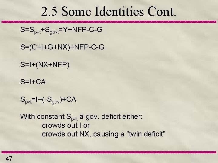
2. 5 Some Identities Cont. S=Spvt+Sgovt=Y+NFP-C-G S=(C+I+G+NX)+NFP-C-G S=I+(NX+NFP) S=I+CA Spvt=I+(-Sgov)+CA With constant Spvt a gov. deficit either: crowds out I or crowds out NX, causing a “twin deficit” 47
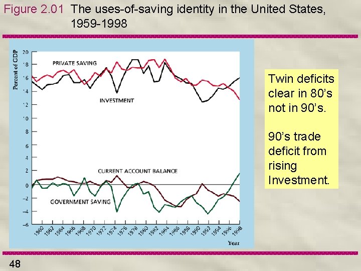
Figure 2. 01 The uses-of-saving identity in the United States, 1959 -1998 Twin deficits clear in 80’s not in 90’s trade deficit from rising Investment. 48

2. 5 Gov and Economy Does gov. borrowing crowd out I or do they both change due to recessions? Classicals: Crowding out Keynesians: Both move in response to Y and aggregate demand. 49
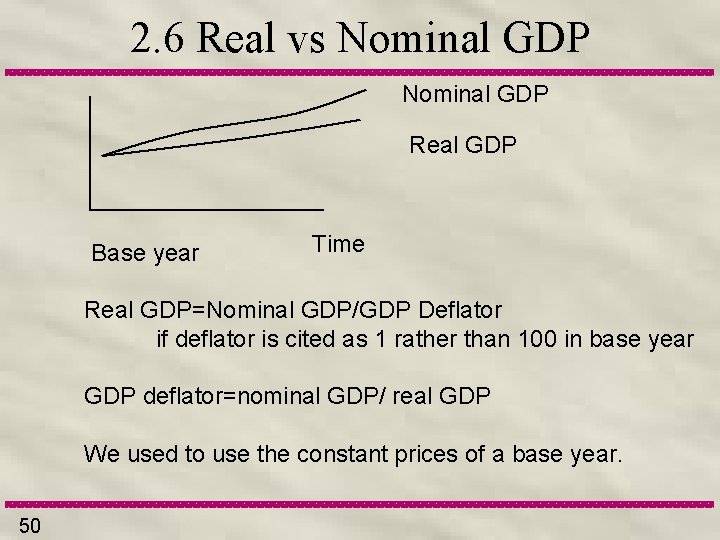
2. 6 Real vs Nominal GDP Real GDP Base year Time Real GDP=Nominal GDP/GDP Deflator if deflator is cited as 1 rather than 100 in base year GDP deflator=nominal GDP/ real GDP We used to use the constant prices of a base year. 50
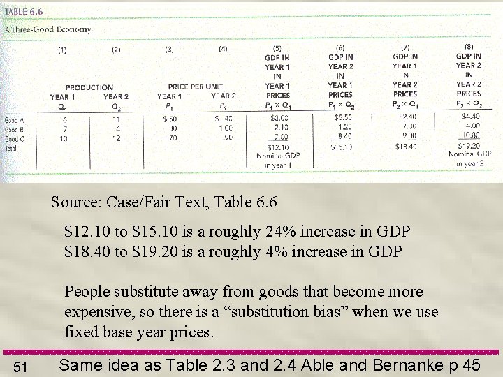
Source: Case/Fair Text, Table 6. 6 $12. 10 to $15. 10 is a roughly 24% increase in GDP $18. 40 to $19. 20 is a roughly 4% increase in GDP People substitute away from goods that become more expensive, so there is a “substitution bias” when we use fixed base year prices. 51 Same idea as Table 2. 3 and 2. 4 Able and Bernanke p 45
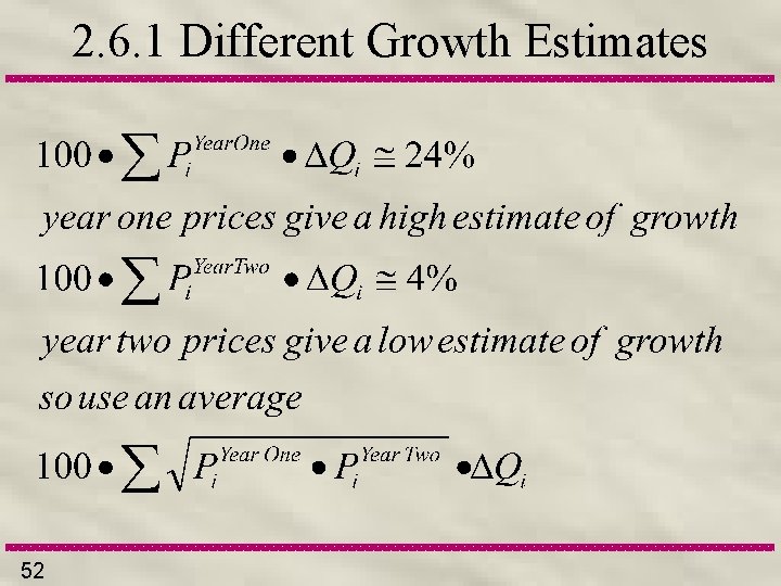
2. 6. 1 Different Growth Estimates 52
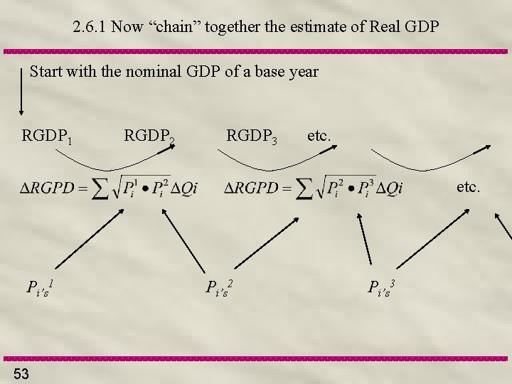
2. 6. 1 Now “chain” together the estimate of Real GDP Start with the nominal GDP of a base year RGDP 1 RGDP 2 RGDP 3 etc. Pi’s 1 53 Pi’s 2 Pi’s 3
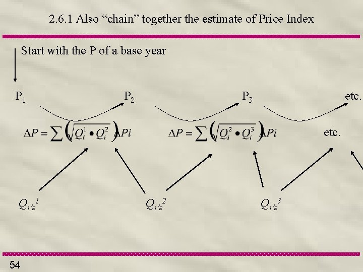
2. 6. 1 Also “chain” together the estimate of Price Index Start with the P of a base year P 1 P 2 P 3 etc. Qi’s 1 54 Qi’s 2 Qi’s 3
2. 6. 1 Chain Type Price Index The “Chain Type” price index for GDP is constructed at the same time by using average baskets from adjacent years to calculate the change in the price level. 55
2. 6. 2 Hedonic Methods NIPA uses “hedonic” methods Goods are separated into characteristics Each characteristic is then priced and tracked It’s not a computer its 256 k. Ram, 20 MB drive…. This does not solve the problem of fundamentally new goods which need to be initially entered at cost. See Krugman on Viagra 56
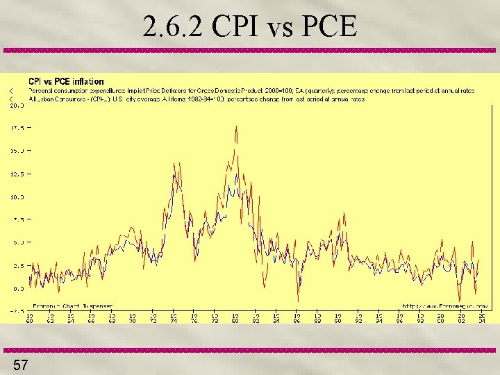
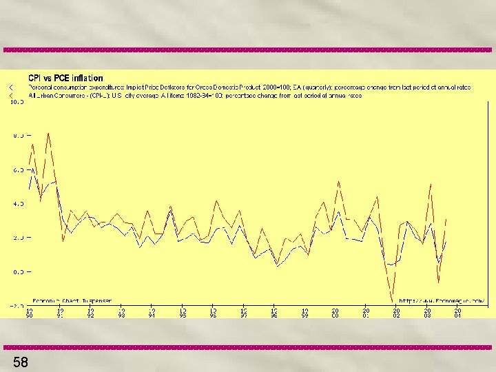
2. 6. 2 CPI vs PCE 57
58
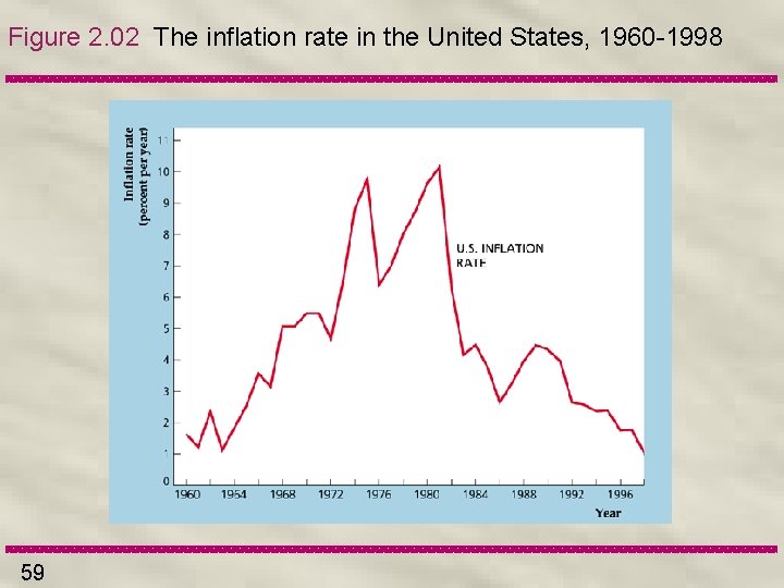
Figure 2. 02 The inflation rate in the United States, 1960 -1998 59
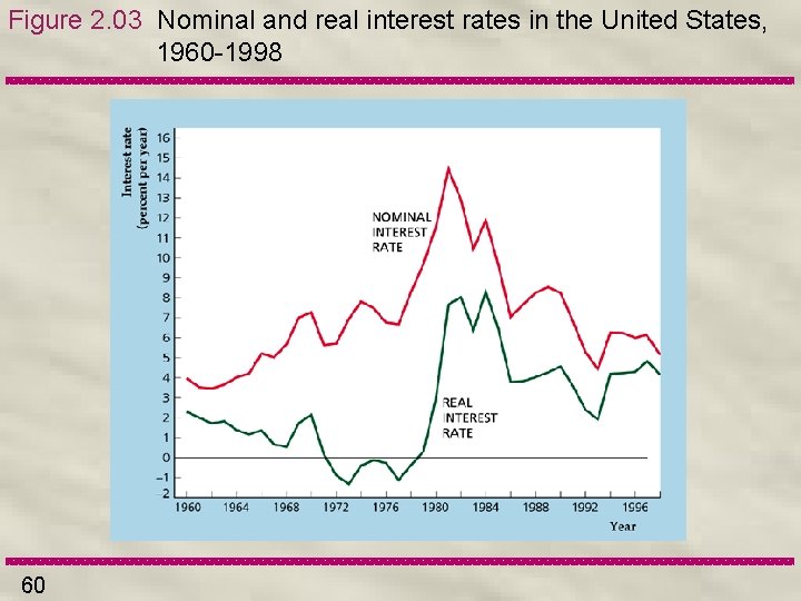
Figure 2. 03 Nominal and real interest rates in the United States, 1960 -1998 60

Extension Topics We may have time for. . GDP vs Well Being Tibor Sciovsky On The Joyless Economy Andrew Oswald on Suicide and Growth Nordhaus on Health and Wealth Social Impact of Downturns GDP components in the 2000 -01 downturn. 61

END & FOR NEXT WEEK Read: Ch 1, Ch 2, Ch 3 and Ch 4 Read: Math Appendix to Book 62
- Slides: 62