VortexScale Hurricane Data Assimilation Preliminary Results with Airborne

Vortex-Scale Hurricane Data Assimilation: Preliminary Results with Airborne Doppler Radar and Dropsondes Using NOAA/AOML/HRD’s HWRF Ensemble Data Assimilation System (HEDAS) Altuğ Aksoy 1, 2 2 U. 1 NOAA/AOML Hurricane Research Division Miami RSMAS Coop. Inst. Marine Atmos. Studies Collaborators: Tomislava Vukicevic, Kathryn Sellwood, Sylvie Lorsolo, Gopal, Jun Zhang, Sim Aberson, and Fuqing Zhang (Penn State)

A Pathway from Research to Operations: HRD’s Strategy • HRD’s main strength and focus is on improving our understanding of hurricane inner-core structure through observations • Quantitative and objective assessment of observation impact can best be done within a data assimilation (DA) framework • HRD began investing in an ensemble-based DA system in the summer of 2008: – Preliminary HEDAS coding and system design completed today – testing continues with observation system simulation experiments (OSSEs) – Real data acquisition and pre-processing systems for airborn Doppler radar and dropsondes underway • System will be tested semi-real-time on NOAA’s n. Jet computer as part of the NOAA HFIP demo system • Systematic, quantitative comparison between 3 DVAR (GSI) and En. KF (collaboration between EMC & HRD): – Analyze differences, identify situations where one or the other system has advantages – Set the foundations for a hybrid VAR-ensemble system

How Can HEDAS Research Provide Feedback to Operational HWRF? • Transition to a common code repository encourages deeper collaboration and quicker code development • HEDAS will provide a natural framework to evaluate model performance and diagnose model structure in observation space • Numerous ensemble- and TC-structure-related diagnostic tools will be contributed to the repository • Ensemble framework will enable a straightforward objective evaluation of model error: – Analysis of growing modes and error growth characteristics – Evaluation of physics schemes through parameter perturbations • Airborne observations will enable the objective initialization of inner-core TC structure

NOAA/AOML/HRD’s HWRF Ensemble Data Assimilation System (HEDAS) • Forecast model: – Experimental Hurricane WRF (HWRF-X) – 2 nested domains (9/3 km horizontal resolution, 42 vert. levels) – Static inner nest to accommodate covariance computations – Ferrier microphysics, explicit convection on inner nest • Ensemble system: – Currently initialized from GEFS ensemble member analyses – 30 ensemble members • Data assimilation: – Square-root En. KF filter (Whitaker and Hamill 2002) – Covariance localization (Gaspari and Cohn 1999) – Assimilates inner-core NOAA P-3 aircraft data on the inner nest

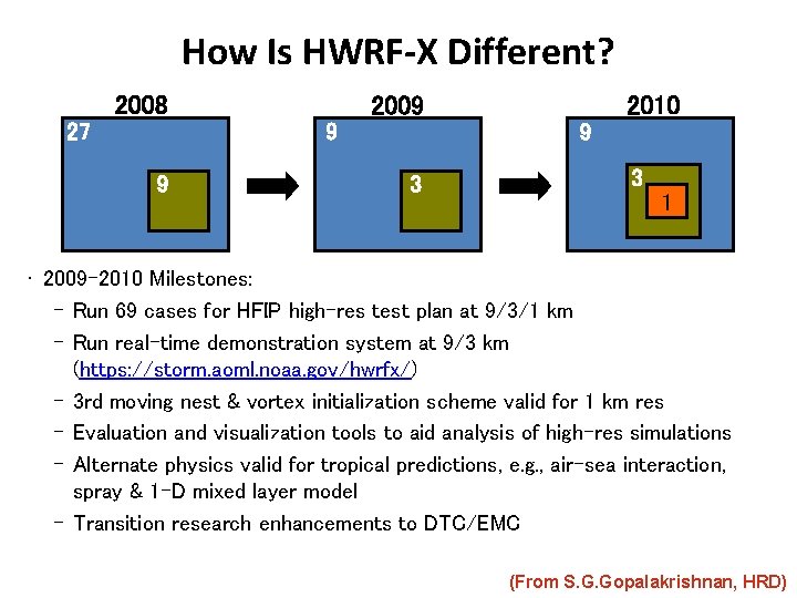
How Is HWRF-X Different? 2008 27 9 9 2010 2009 9 3 3 1 • 2009 -2010 Milestones: – Run 69 cases for HFIP high-res test plan at 9/3/1 km – Run real-time demonstration system at 9/3 km (https: //storm. aoml. noaa. gov/hwrfx/) – 3 rd moving nest & vortex initialization scheme valid for 1 km res – Evaluation and visualization tools to aid analysis of high-res simulations – Alternate physics valid for tropical predictions, e. g. , air-sea interaction, spray & 1 -D mixed layer model – Transition research enhancements to DTC/EMC (From S. G. Gopalakrishnan, HRD)

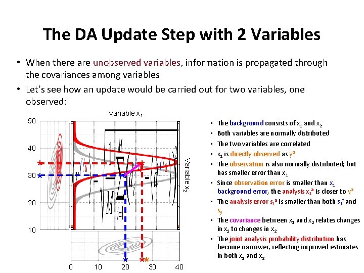
The DA Update Step with 2 Variables • When there are unobserved variables, information is propagated through the covariances among variables • Let’s see how an update would be carried out for two variables, one observed: Variable x 1 50 40 * * Variable x 2 * 30 * • • 20 • 10 • 0 10 * **30 20 40 The background consists of x 1 and x 2 Both variables are normally distributed The two variables are correlated x 1 is directly observed as y 0 The observation is also normally distributed; but has smaller error than x 1 Since observation error is smaller than x 1 background error, the analysis x 1 a is closer to y 0 The analysis error s 1 a is smaller than both s 1 f and sy The covariance between x 1 and x 2 relates changes in x 1 to changes in x 2 The joint analysis probability distribution has become narrower, reflecting improved estimates in both x 1 and x 2

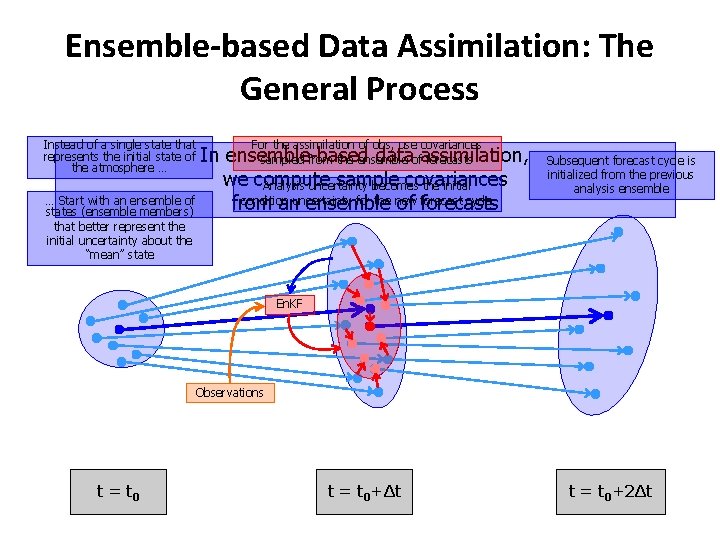
Ensemble-based Data Assimilation: The General Process Instead of a single state that represents the initial state of the atmosphere … … Start with an ensemble of states (ensemble members) that better represent the initial uncertainty about the “mean” state For the assimilation of obs, use covariances In ensemble-based dataofassimilation, sampled from the ensemble forecasts we compute sample covariances Analysis uncertainty becomes the initial condition for the new forecast cycle from anuncertainty ensemble of forecasts Subsequent forecast cycle is initialized from the previous analysis ensemble En. KF Observations t = t 0+Δt t = t 0+2Δt

Advantages of Ensemble-based Data Assimilation • Background covariances are sampled from the forecast ensemble → Flow-dependent covariances that are independent of any assumptions for the nature of flow (e. g. , geostrophy) • Provides a natural basis for probabilistic forecasts • Easy to implement and maintain • No adjoints are needed to be developed which is especially complicated for highly nonlinear and discontinuous sub-grid parameterization schemes and/or nonlinear observation operators • Straightforward application to domains with multiple nests • Easily lends itself to parallelization • Performance (so far) comparable to variational schemes

HEDAS System Characteristics • En. KF system coded in Fortran 90 • Critical parts of En. KF code parallelized using Open. MP architecture: • Relatively simple design • Shared-memory architecture of Open. MP allows for minimal exchange among computational threads • Limited to parallelization on a single node (n. Jet allows for 8 threads per node) • Real data acquisition will be done through operational channels: Currently planning to assimilate airborne Doppler wind, dropsonde, and flight-level data • Wrapper bash script manages work flow during cycling • 30 ensemble members will run on 32 nodes/member in parallel (~1000 nodes) to maximize benefits of parallelization – only during 4 -6 hr of analysis

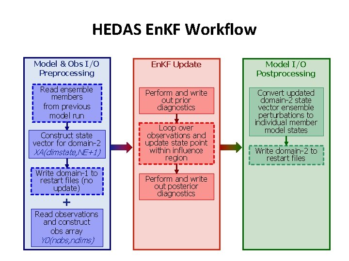
HEDAS En. KF Workflow Model & Obs I/O Preprocessing En. KF Update Model I/O Postprocessing Read ensemble members from previous model run Perform and write out prior diagnostics Construct state vector for domain-2 Loop over observations and update state point within influence region Convert updated domain-2 state vector ensemble perturbations to individual member model states XA(dimstate, NE+1) Write domain-1 to restart files (no update) + Read observations and construct obs array Y 0(nobs, ndims) Perform and write out posterior diagnostics Write domain-2 to restart files

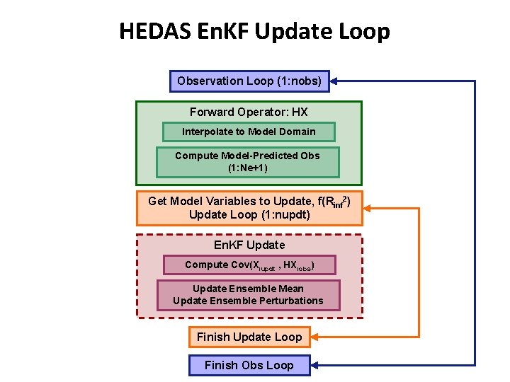
HEDAS En. KF Update Loop Observation Loop (1: nobs) Forward Operator: HX Interpolate to Model Domain Compute Model-Predicted Obs (1: Ne+1) Get Model Variables to Update, f(Rinf 2) Update Loop (1: nupdt) En. KF Update Compute Cov(Xiupdt , HXiobs) Update Ensemble Mean Update Ensemble Perturbations Finish Update Loop Finish Obs Loop

NOAA Operates Three Aircraft to Observe Hurricane Environment and Vortex Structure: P-3 Aircraft (eye penetrations) GPS Humidity Chemistry inlet Radar altimeter Gust probe Tail Doppler Radar C-Band Weather Radar Pylons Radiometer Lower-fuselage Weather Radar HRD En. KF Effort Primarily Focusing on Dropsonde, Doppler Radar, and Flight-Level Obs Launch tubes and chutes: Dropwindsonde, AXBT, AXCP, AXCTD (Stepped-frequency Microwave Radiometer, cloud physics, aerosol) GPS navigation G-IV Aircraft (environmental) Tail Doppler Radar (new) C-Band Weather Radar Stepped-frequency Microwave Radiometer Dropwindsonde chute

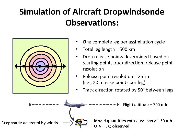
Simulation of Aircraft Dropwindsonde Observations: • One complete leg per assimilation cycle • Total leg length = 500 km • Drop release points determined based on starting point, track direction, release point resolution • Release point resolution = 25 km (i. e. , 20 release points per leg) • Track direction rotated by 50° between legs Flight altitude = 700 mb Dropsonde advected by winds Model quantities extracted every ~ 50 mb U, V, T, Q observed

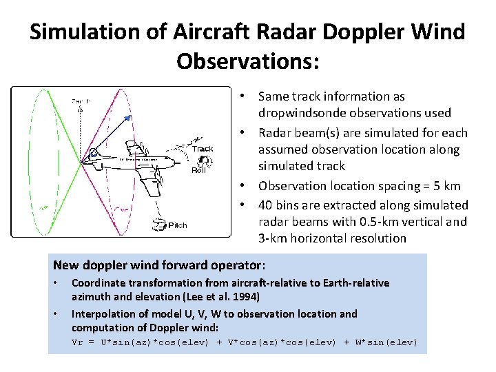
Simulation of Aircraft Radar Doppler Wind Observations: • Same track information as dropwindsonde observations used • Radar beam(s) are simulated for each assumed observation location along simulated track • Observation location spacing = 5 km • 40 bins are extracted along simulated radar beams with 0. 5 -km vertical and 3 -km horizontal resolution New doppler wind forward operator: • • Coordinate transformation from aircraft-relative to Earth-relative azimuth and elevation (Lee et al. 1994) Interpolation of model U, V, W to observation location and computation of Doppler wind: Vr = U*sin(az)*cos(elev) + V*cos(az)*cos(elev) + W*sin(elev)

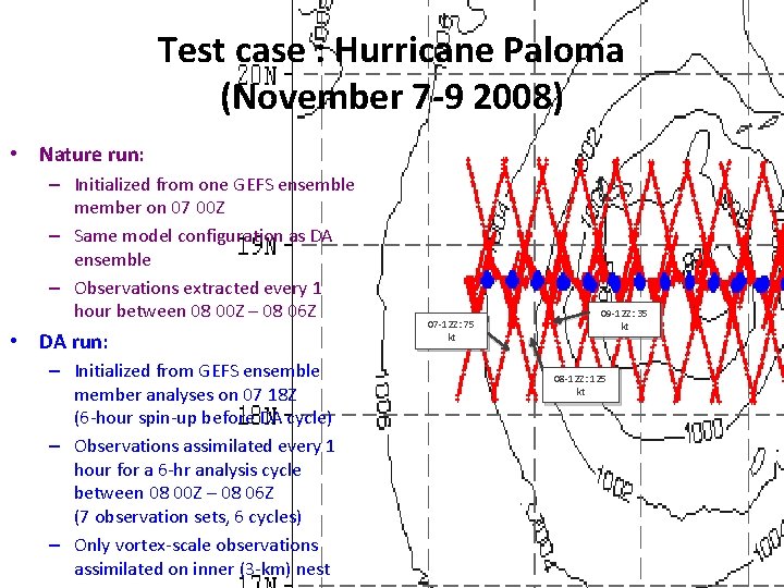
Test case : Hurricane Paloma (November 7 -9 2008) • Nature run: – Initialized from one GEFS ensemble member on 07 00 Z – Same model configuration as DA ensemble – Observations extracted every 1 hour between 08 00 Z – 08 06 Z • DA run: – Initialized from GEFS ensemble member analyses on 07 18 Z (6 -hour spin-up before DA cycle) – Observations assimilated every 1 hour for a 6 -hr analysis cycle between 08 00 Z – 08 06 Z (7 observation sets, 6 cycles) – Only vortex-scale observations assimilated on inner (3 -km) nest 07 -12 Z: 75 kt 09 -12 Z: 35 kt 08 -12 Z: 125 kt

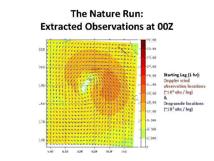
The Nature Run: Extracted Observations at 00 Z Starting Leg (1 hr): Doppler wind observation locations (~104 obs / leg) & Dropsonde locations (~103 obs / leg)

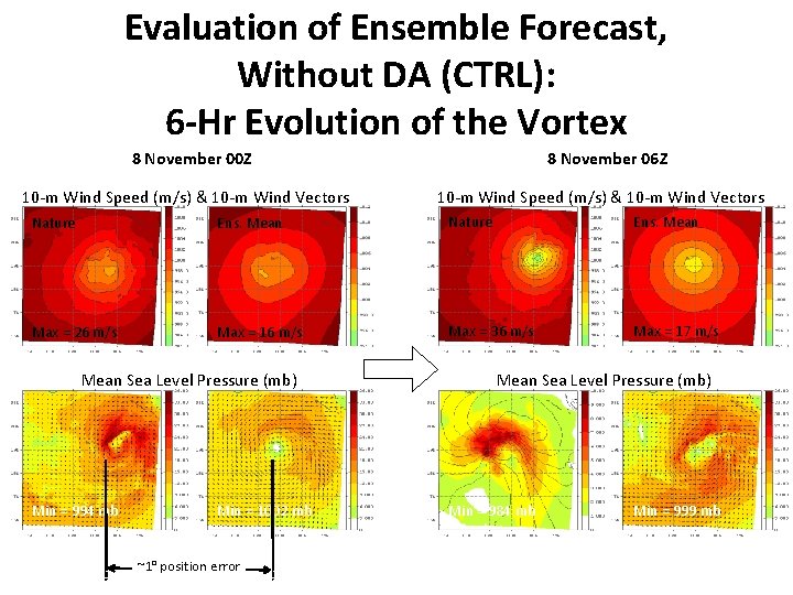
Evaluation of Ensemble Forecast, Without DA (CTRL): 6 -Hr Evolution of the Vortex 8 November 00 Z 10 -m Wind Speed (m/s) & 10 -m Wind Vectors 8 November 06 Z 10 -m Wind Speed (m/s) & 10 -m Wind Vectors Nature Ens. Mean Max = 26 m/s Max = 16 m/s Max = 36 m/s Max = 17 m/s Mean Sea Level Pressure (mb) Min = 994 mb Min = 1002 mb ~1° position error Mean Sea Level Pressure (mb) Min = 984 mb Min = 999 mb

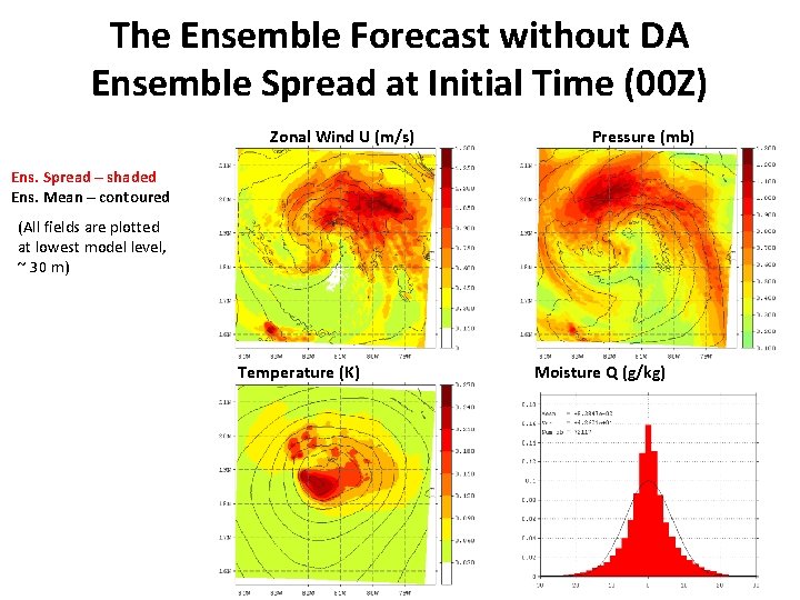
The Ensemble Forecast without DA Ensemble Spread at Initial Time (00 Z) Zonal Wind U (m/s) Pressure (mb) Ens. Spread – shaded Ens. Mean – contoured (All fields are plotted at lowest model level, ~ 30 m) Temperature (K) Moisture Q (g/kg)

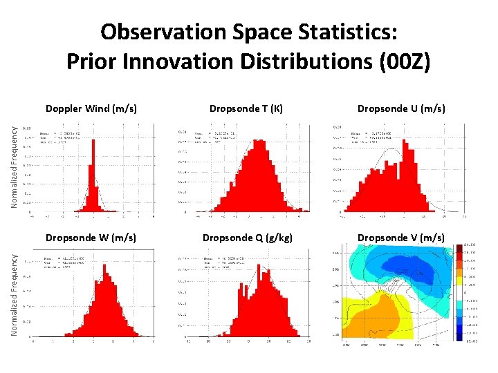
Observation Space Statistics: Prior Innovation Distributions (00 Z) Dropsonde T (K) Dropsonde U (m/s) Dropsonde W (m/s) Dropsonde Q (g/kg) Dropsonde V (m/s) Normalized Frequency Doppler Wind (m/s)

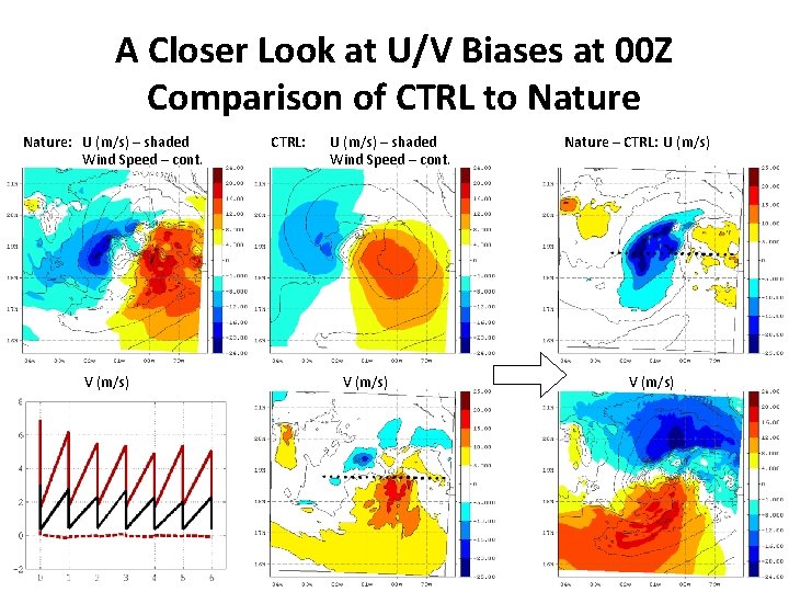
A Closer Look at U/V Biases at 00 Z Comparison of CTRL to Nature: U (m/s) – shaded Wind Speed – cont. V (m/s) CTRL: U (m/s) – shaded Wind Speed – cont. V (m/s) Nature – CTRL: U (m/s) V (m/s)

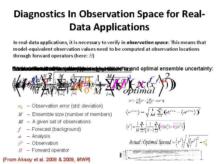
Diagnostics In Observation Space for Real. Data Applications In real-data applications, it is necessary to verify in observation space: This means that model-equivalent observation values need to be computed at observation locations through forward operators (here: H) Forecast “ensemble is: spread Random forecast error is explained by obs error and optimal ensemble uncertainty: Let’s the“root-mean innovation as: “Mean Innovation” is spread” domain-averaged bias: Bias-corrected So wedefine can define “actual/optimal square innovation” ratio” is: as: σ0 – Observation error (std. deviation) N – Ensemble size (number of members) M – A given set of observations f a y 0 H – – Forecast (background) Analysis Observation Forward operator (From Aksoy et al. 2008 & 2009, MWR)

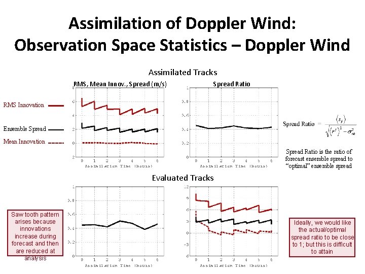
Assimilation of Doppler Wind: Observation Space Statistics – Doppler Wind Assimilated Tracks RMS, Mean Innov. , Spread (m/s) Spread Ratio RMS Innovation Ensemble Spread Mean Innovation Assimilation Time (hours) Spread Ratio is the ratio of forecast ensemble spread to “optimal” ensemble spread Evaluated Tracks Saw tooth pattern arises because innovations increase during forecast and then are reduced at analysis Ideally, we would like the actual/optimal spread ratio to be close to 1; but this is difficult to attain Assimilation Time (hours)

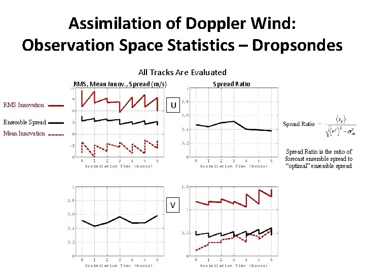
Assimilation of Doppler Wind: Observation Space Statistics – Dropsondes All Tracks Are Evaluated RMS, Mean Innov. , Spread (m/s) Spread Ratio U RMS Innovation Ensemble Spread Mean Innovation Assimilation Time (hours) V Assimilation Time (hours) Spread Ratio is the ratio of forecast ensemble spread to “optimal” ensemble spread

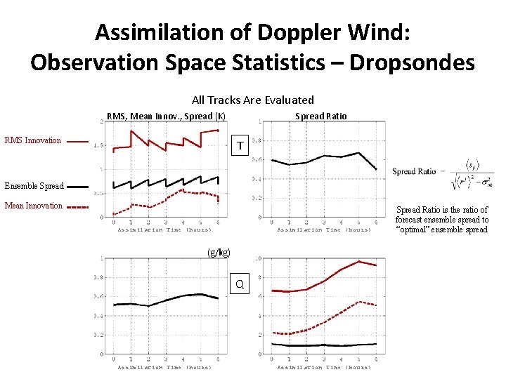
Assimilation of Doppler Wind: Observation Space Statistics – Dropsondes All Tracks Are Evaluated RMS, Mean Innov. , Spread (K) RMS Innovation Spread Ratio T Ensemble Spread Mean Innovation Assimilation Time (hours) (g/kg) Q Assimilation Time (hours) Spread Ratio is the ratio of forecast ensemble spread to “optimal” ensemble spread

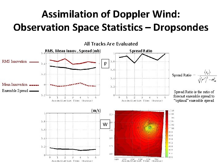
Assimilation of Doppler Wind: Observation Space Statistics – Dropsondes All Tracks Are Evaluated RMS, Mean Innov. , Spread (mb) RMS Innovation Spread Ratio P Mean Innovation Ensemble Spread Assimilation Time (hours) (m/s) W Assimilation Time (hours) Spread Ratio is the ratio of forecast ensemble spread to “optimal” ensemble spread

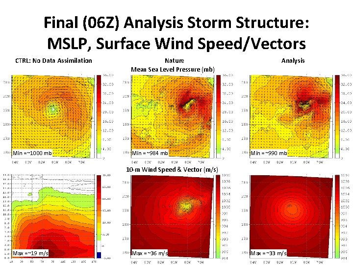
Final (06 Z) Analysis Storm Structure: MSLP, Surface Wind Speed/Vectors CTRL: No Data Assimilation Min = ~1000 mb Nature Mean Sea Level Pressure (mb) Min = ~984 mb Analysis Min = ~990 mb 10 -m Wind Speed & Vector (m/s) Max = ~19 m/s Max = ~36 m/s Max = ~33 m/s

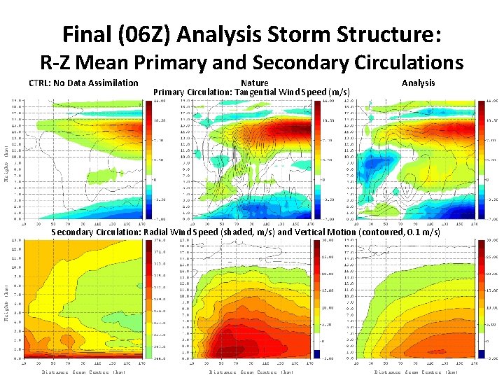
Final (06 Z) Analysis Storm Structure: R-Z Mean Primary and Secondary Circulations Nature Primary Circulation: Tangential Wind Speed (m/s) Analysis Height (km) CTRL: No Data Assimilation Height (km) Secondary Circulation: Radial Wind Speed (shaded, m/s) and Vertical Motion (contoured, 0. 1 m/s) Distance from Center (km)

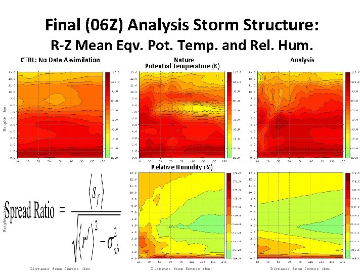
Final (06 Z) Analysis Storm Structure: R-Z Mean Eqv. Pot. Temp. and Rel. Hum. Nature Potential Temperature (K) Analysis Height (km) CTRL: No Data Assimilation Height (km) Relative Humidity (%) Distance from Center (km)

Why Does Ensemble Spread Matter in Data Assimilation? • Ensemble spread, or what is technically called prior (background) variance, determines how much confidence we have in our prior (background) state estimate • When ensemble spread is smaller than observation error, the DA system interpretes that as “there is more confidence in the background than in the observation” • The smaller the ensemble spread, the less impact an observation will have on the background • We run the danger that the ensemble mean will begin to drift away from the observations (filter divergence)

How Can We Improve Ensemble Spread? • Sampling errors due to limited size of ensemble tend to result in underestimation of background errors • Optimize covariance localization to balance the number of observations that update each model grid point • Implement covariance inflation (various techniques available) • Ensemble variability should ideally also encompass model error; under-representation of model error will lead to spread deficiency • Initial perturbations should ideally project on the growing modes of the model • Perturbed-parameter ensembles that target critical parts of parameterization schemes allow for straightforward representation of model error

HEDAS Strategy to Approach the Ensemble Spread Problem • Experimentation with GFS-En. KF initial/boundary conditions • • More ensemble members (60 available) Higher resolution (0. 5 degree analysis data) Calibrated ensemble spread More frequently available (every 1 hr) • Experimentation with perturbed-parameter model physics • Infrastructure completed to incorporate perturbed HWRF parameters across ensemble members • Initially targeting surface-layer momentum and heat exchange coefficients

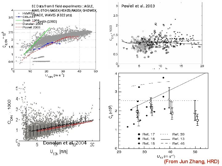
EC Data from 8 field experiments : AGILE, AWE, ETCH, GASEX, HEXOS, RASEX, SHOWEX, SWADE, WAVES (4322 pts). Powell et al. 2003 — Smith (1980) Donelan et al. 2004 (From Jun Zhang, HRD)

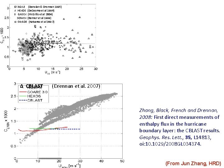
O AGILE (Donelan & Drennan 1995) X HEXOS (De. Cosmo et al 1996) ◊ GASEX (Mc. Gillis et al 2004) SOWEX (Banner et al 1999) □ SWADE (Katsaros et al 1993) Δ CBLAST COARE-3 --COARE 2. 5 — (Drennan et al. 2007) Zhang, Black, French and Drennan, 2008: First direct measurements of enthalpy flux in the hurricane boundary layer: the CBLAST results. Geophys. Res. Lett. , 35, L 14813, oi: 10. 1029/2008 GL 034374. (From Jun Zhang, HRD)

Further HEDAS development (Fall/Winter 2010/11) • Full coupling with the global En. SRF system • Assimilate satellite data through GSI operators on the parent nest • Transition to common En. SRF solver • Assimilation of new observation platforms, potentially including ocean data (SFMR, LIDAR, AXBTs, etc. ) • Diagnostics and assimilation of satellite data in the innercore region • Model error related parameter estimation • Experimentation with non-linear update techniques • Experimentation with storm-centered covariances and filter updates • Code enhancements and more parallelization

The End