Volume Graphics lecture 5 Contour Tree Contour Spectrum

Volume Graphics (lecture 5 : Contour Tree / Contour Spectrum) lecture notes acknowledgement : J. Snoeyink, C. Bajaj Bong-Soo Sohn School of Computer Science and Engineering Chung-Ang University

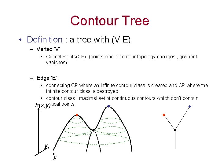
Contour Tree • Definition : a tree with (V, E) – Vertex ‘V’ • Critical Points(CP) (points where contour topology changes , gradient vanishes) – Edge ‘E’: • connecting CP where an infinite contour class is created and CP where the infinite contour class is destroyed. • contour class : maximal set of continuous contours which don’t contain critical points h(x, y) y x

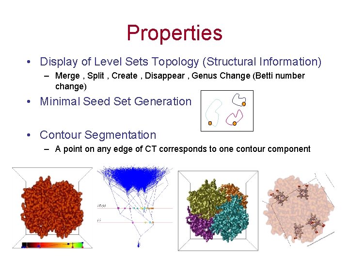
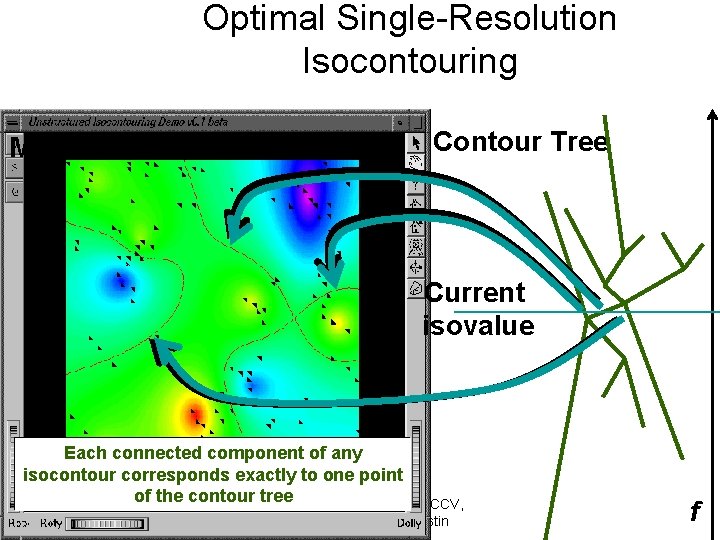
Properties • Display of Level Sets Topology (Structural Information) – Merge , Split , Create , Disappear , Genus Change (Betti number change) • Minimal Seed Set Generation • Contour Segmentation – A point on any edge of CT corresponds to one contour component

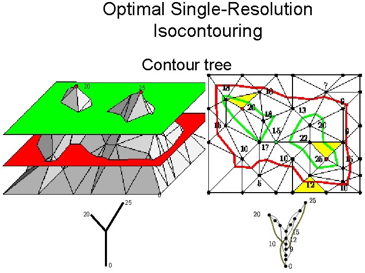
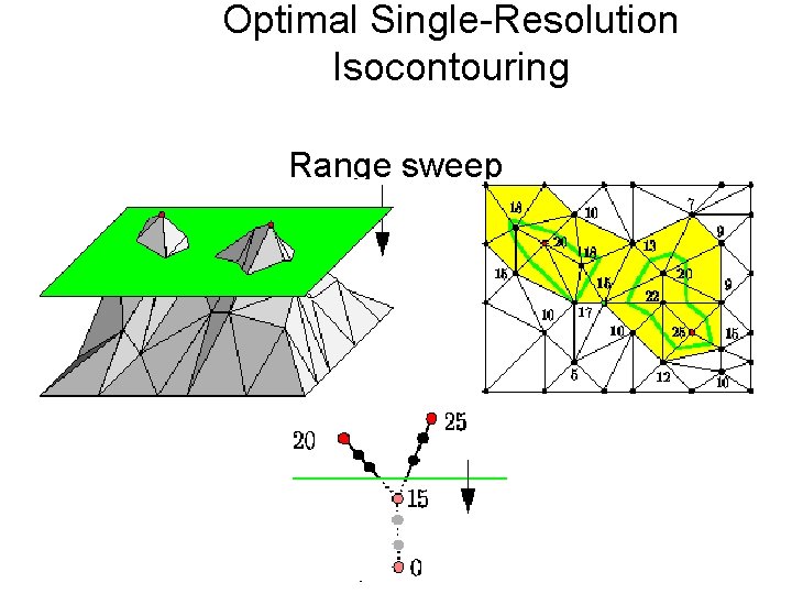
Optimal Single-Resolution Isocontouring Contour tree 20 25 20 0

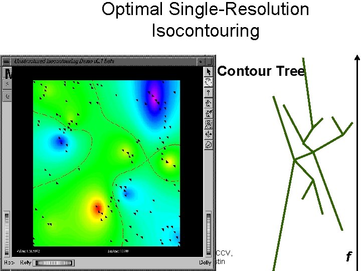
Optimal Single-Resolution Isocontouring Minimal Seed Set Contour Tree Copyright: Chandrajit Bajaj, CCV, University of Texas at Austin f

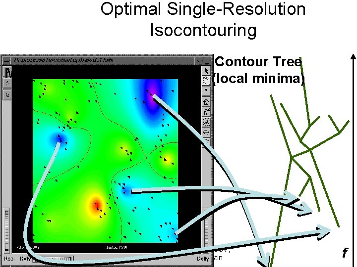
Optimal Single-Resolution Isocontouring Minimal Seed Set Contour Tree (local minima) Copyright: Chandrajit Bajaj, CCV, University of Texas at Austin f

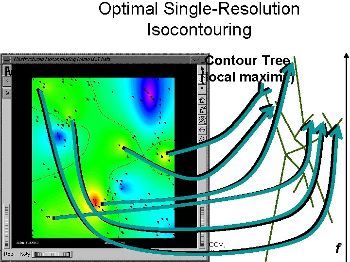
Optimal Single-Resolution Isocontouring Minimal Seed Set Contour Tree (local maxima) Copyright: Chandrajit Bajaj, CCV, University of Texas at Austin f

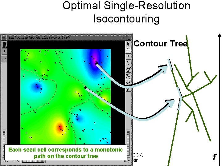
Optimal Single-Resolution Isocontouring Minimal Seed Set Contour Tree Each seed cell corresponds to a monotonic Copyright: path on the contour tree Chandrajit Bajaj, CCV, University of Texas at Austin f

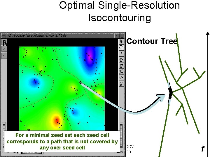
Optimal Single-Resolution Isocontouring Minimal Seed Set Contour Tree For a minimal seed set each seed cell corresponds to a path that is not covered by Chandrajit Bajaj, CCV, any over seed. Copyright: cell University of Texas at Austin f

Optimal Single-Resolution Isocontouring Minimal Seed Set Contour Tree Current isovalue Each connected component of any isocontour corresponds exactly to one point of the contour Copyright: tree Chandrajit Bajaj, CCV, University of Texas at Austin f

Optimal Single-Resolution Isocontouring Range sweep Copyright: Chandrajit Bajaj, CCV, University of Texas at Austin

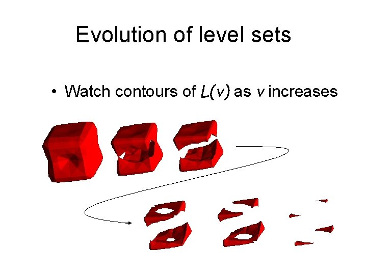
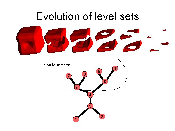
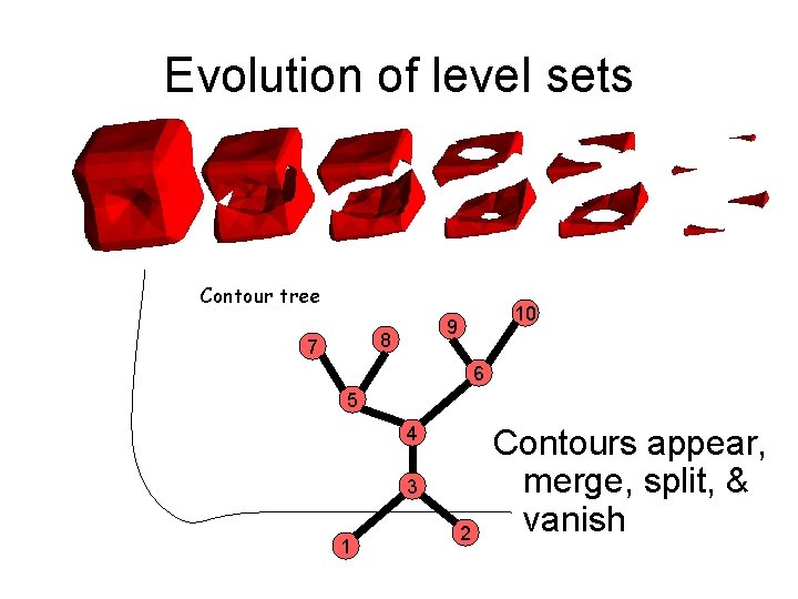
Evolution of level sets • Watch contours of L(v) as v increases

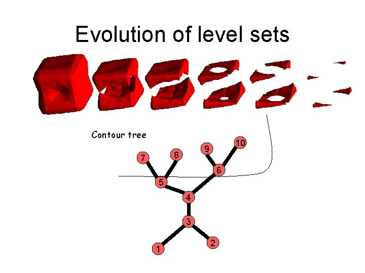
Evolution of level sets Contour tree 8 7 10 9 6 5 4 3 1 2

Evolution of level sets Contour tree 8 7 10 9 6 5 4 3 1 2

Evolution of level sets Contour tree 8 7 10 9 6 5 4 3 1 2

Evolution of level sets Contour tree 8 7 10 9 6 5 4 3 1 2

Evolution of level sets Contour tree 8 7 10 9 6 5 4 3 1 2

Evolution of level sets Contour tree 8 7 10 9 6 5 4 3 1 2 Contours appear, merge, split, & vanish

Morse theory & Contour trees • • Karron et al 95, digital Morse theory Bajaj et al 97– 99, seed sets Van Kreveld et al 97, 2 -D contour tree Tarasov & Vyalyi 98, 3 -D contour tree

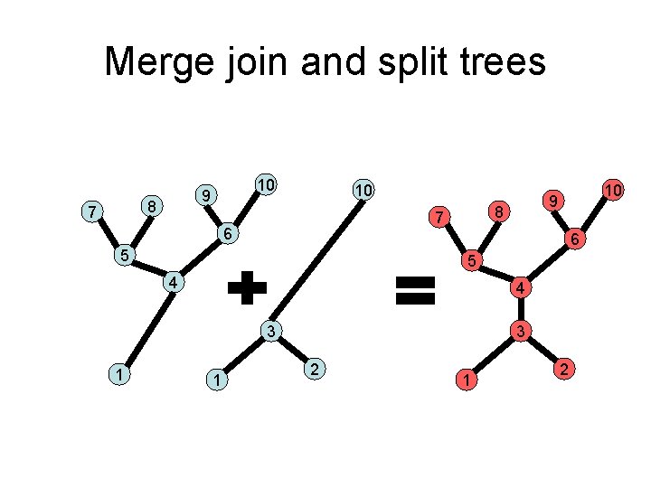
How to compute contour trees without sweeping all level sets • Build join and split trees • Merge to form contour tree • Works in all dimensions. . .

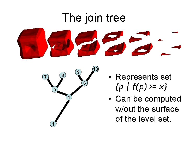
The join tree 8 7 10 9 6 5 4 1 • Represents set {p | f(p) >= x} • Can be computed w/out the surface of the level set.

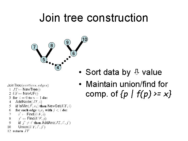
Join tree construction 8 7 10 9 6 5 4 • Sort data by value • Maintain union/find for comp. of {p | f(p) >= x}

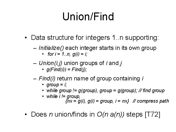
Union/Find • Data structure for integers 1. . n supporting: – Initialize() each integer starts in its own group • for i = 1. . n, g(i) = i; – Union(i, j) union groups of i and j • g(Find(i)) = Find(j); – Find(i) return name of group containing i • group = i; • while group != g(group), group = g(group); // find group • while i != group, {nx = g(i), g(i) = group, i = nx} // compress path • Does n union/finds in O(n a(n)) steps [T 72]

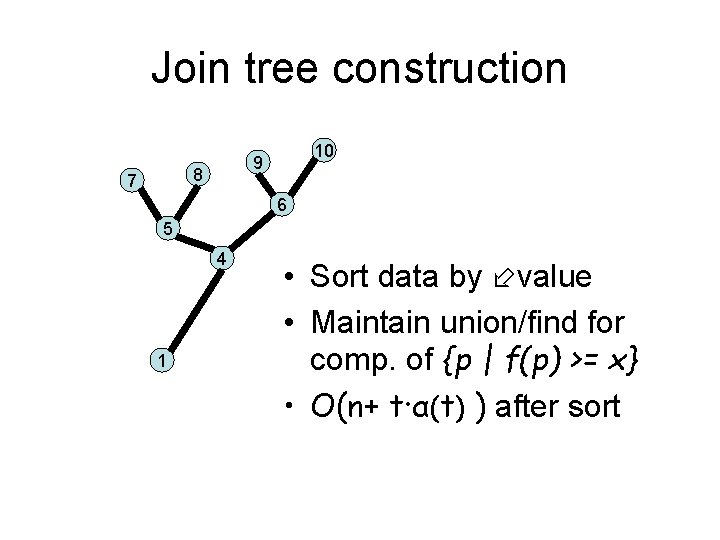
Join tree construction 8 7 10 9 6 5 4 1 • Sort data by value • Maintain union/find for comp. of {p | f(p) >= x} • O(n+ t·α(t) ) after sort

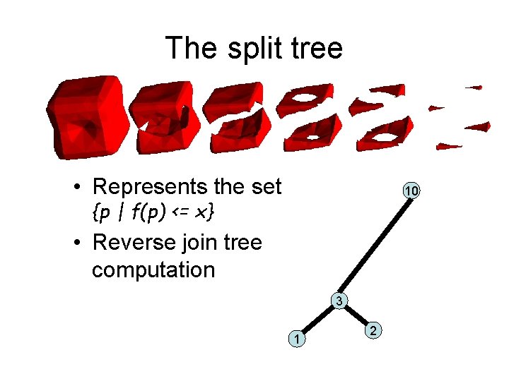
The split tree • Represents the set 10 {p | f(p) <= x} • Reverse join tree computation 3 1 2

Merge join and split trees 8 7 10 9 10 8 7 6 6 5 5 4 4 3 1 10 9 1 3 2 1 2

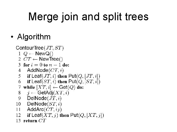
Merge join and split trees • Algorithm

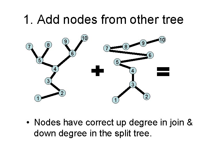
1. Add nodes from other tree 8 7 10 9 6 5 8 7 6 5 4 4 3 1 10 9 3 2 1 2 • Nodes have correct up degree in join & down degree in the split tree.

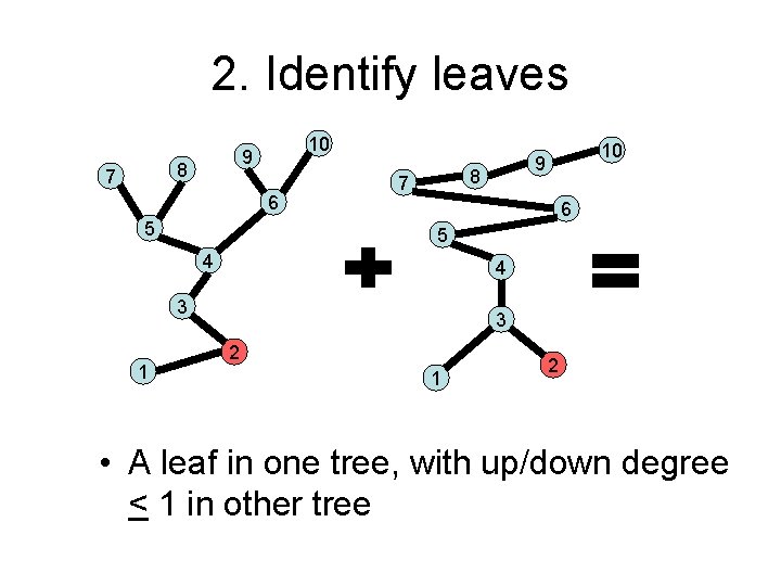
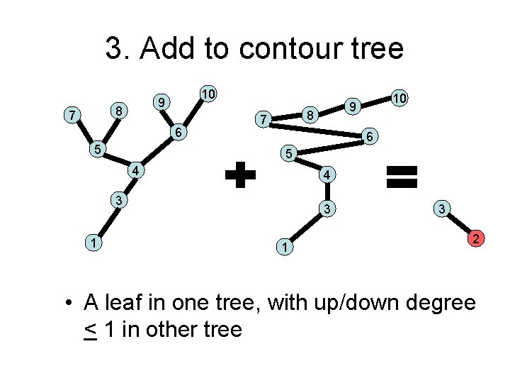
2. Identify leaves 8 7 10 9 6 5 8 7 6 5 4 4 3 1 10 9 3 2 1 2 • A leaf in one tree, with up/down degree < 1 in other tree

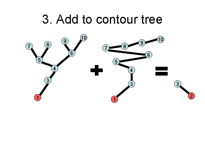
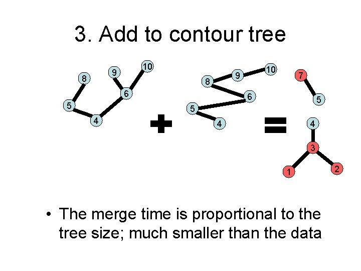
3. Add to contour tree 8 7 10 9 6 5 8 7 6 5 4 4 3 1 10 9 3 1 3 2 • A leaf in one tree, with up/down degree < 1 in other tree

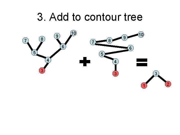
3. Add to contour tree 8 7 10 9 6 5 8 7 6 5 4 4 3 1 10 9 3 1 3 2

3. Add to contour tree 8 7 10 9 6 5 4 3 3 1 2

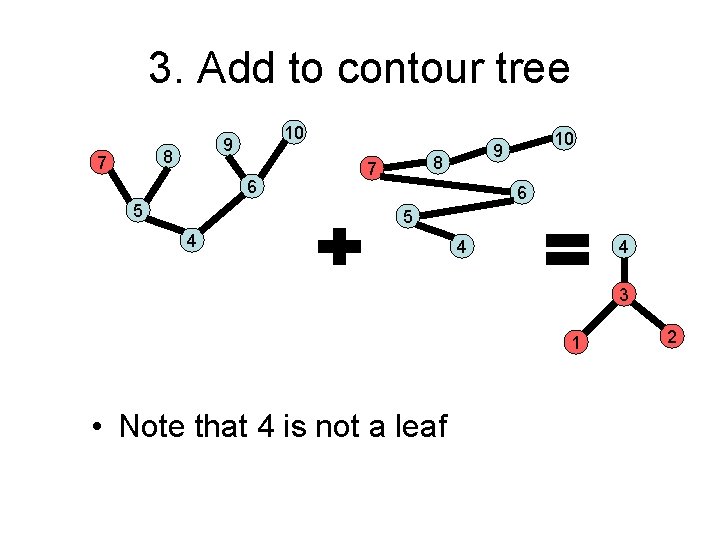
3. Add to contour tree 8 7 10 9 6 5 4 4 4 3 1 • Note that 4 is not a leaf 2

3. Add to contour tree 10 9 8 8 6 5 10 9 7 6 5 5 4 4 4 3 1 • The merge time is proportional to the tree size; much smaller than the data 2

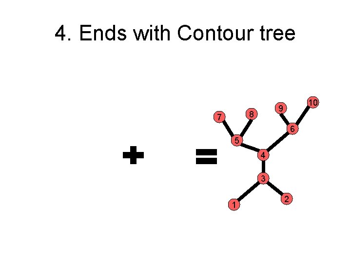
4. Ends with Contour tree 8 7 10 9 6 5 4 3 1 2

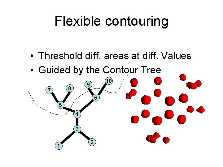
Advantages • Doesn’t need the surface structure to build the contour tree. • The merge becomes simple, and works on a subset of the points • The tree structure can advise where to choose threshold value • Can cut diff. branches at diff. values.

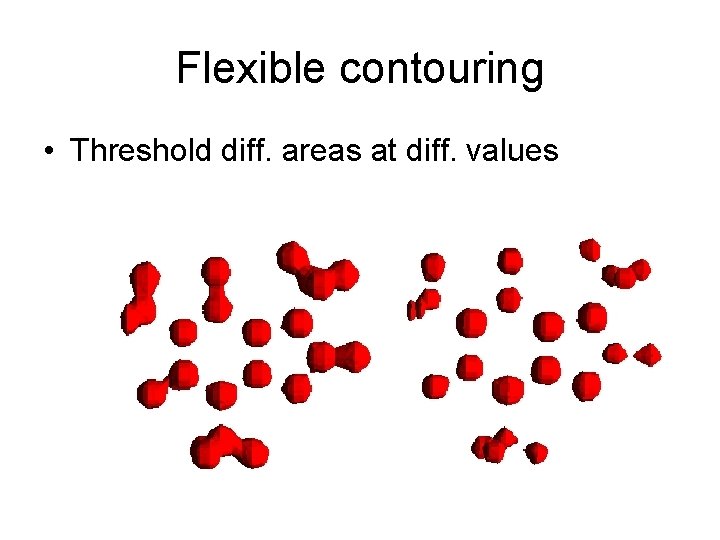
Flexible contouring • Threshold diff. areas at diff. values

Flexible contouring • Threshold diff. areas at diff. Values • Guided by the Contour Tree 8 7 10 9 6 5 4 3 1 2

Contour Spectrum • • • User Interface Signature Computation Real Time Quantitative Queries Topological Information Semi-Automatic Isovalue Selection

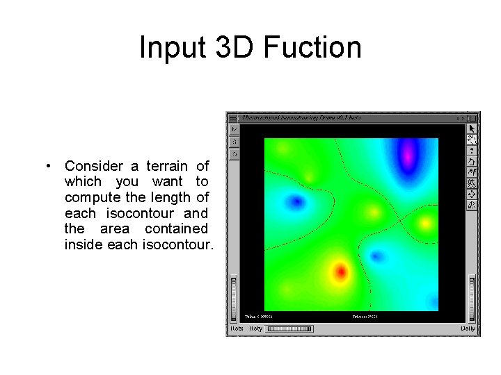
Input 3 D Fuction • Consider a terrain of which you want to compute the length of each isocontour and the area contained inside each isocontour.

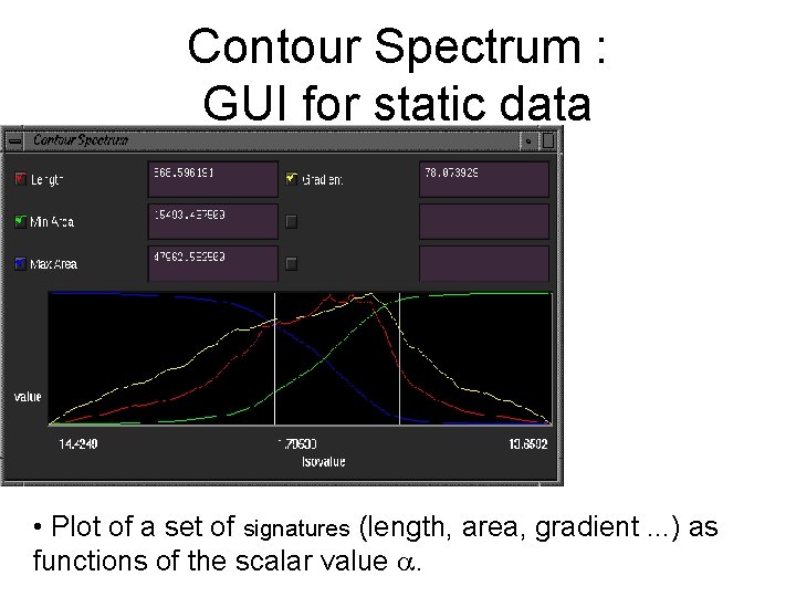
Contour Spectrum : GUI for static data • Plot of a set of signatures (length, area, gradient. . . ) as functions of the scalar value .

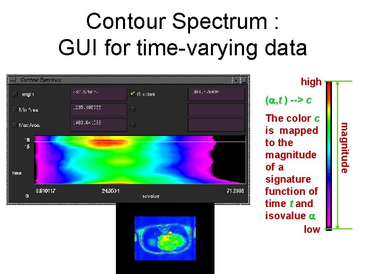
Contour Spectrum : GUI for time-varying data high ( , t ) --> c magnitude The color c is mapped to the magnitude of a signature function of time t and isovalue low

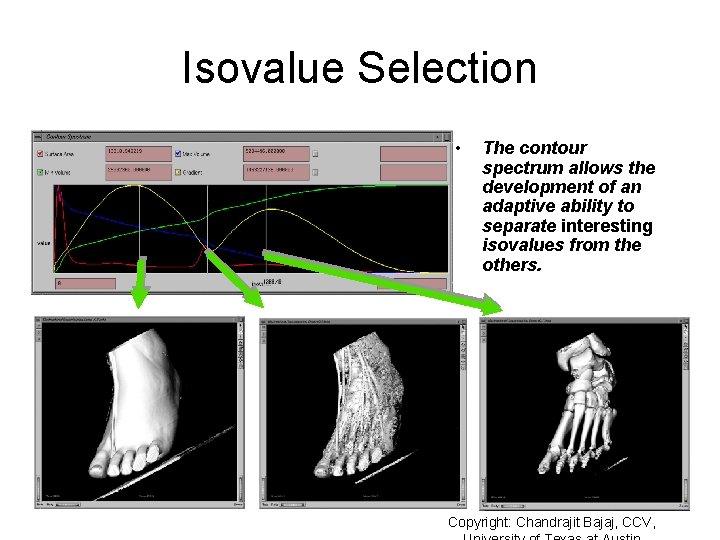
Isovalue Selection • The contour spectrum allows the development of an adaptive ability to separate interesting isovalues from the others. Copyright: Chandrajit Bajaj, CCV,

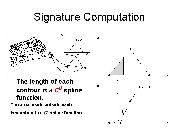
Signature Computation – The length of each contour is a c 0 spline function. The area inside/outside each isocontour is a C 1 spline function.

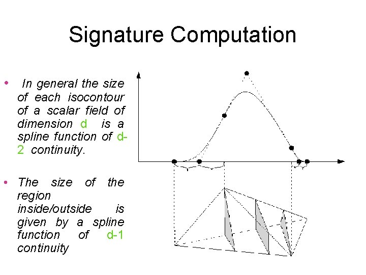
Signature Computation • In general the size of each isocontour of a scalar field of dimension d is a spline function of d 2 continuity. • The size of the region inside/outside is given by a spline function of d-1 continuity