Volume 1 of Parallel Distributed Processing 1986 shows

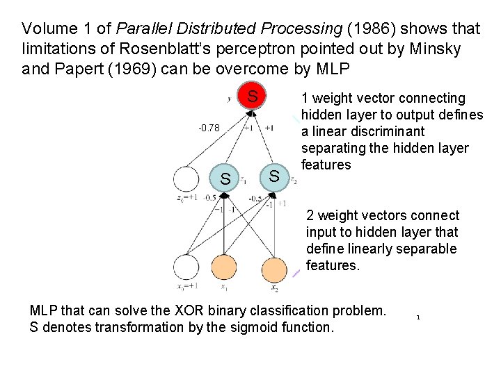
Volume 1 of Parallel Distributed Processing (1986) shows that limitations of Rosenblatt’s perceptron pointed out by Minsky and Papert (1969) can be overcome by MLP S -0. 78 S S 1 weight vector connecting hidden layer to output defines a linear discriminant separating the hidden layer features 2 weight vectors connect input to hidden layer that define linearly separable features. MLP that can solve the XOR binary classification problem. S denotes transformation by the sigmoid function. 1

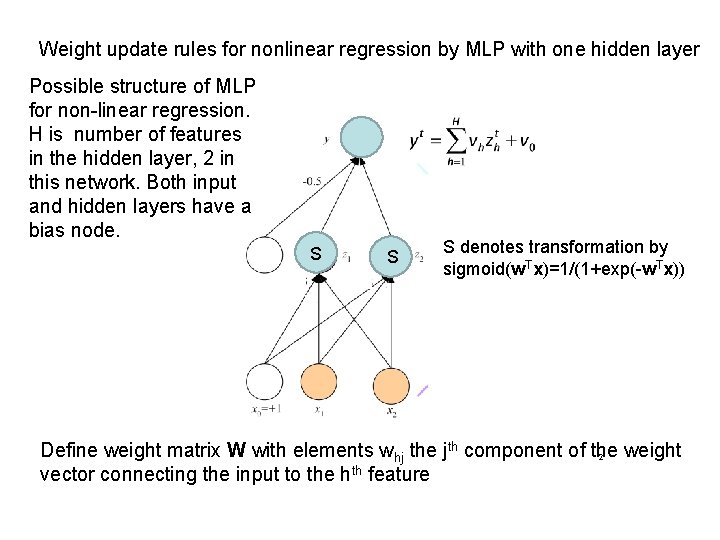
Weight update rules for nonlinear regression by MLP with one hidden layer Possible structure of MLP for non-linear regression. H is number of features in the hidden layer, 2 in this network. Both input and hidden layers have a bias node. S S S denotes transformation by S Tx)=1/(1+exp(-w. Tx)) sigmoid(w Define weight matrix W with elements whj the jth component of the weight 2 vector connecting the input to the hth feature

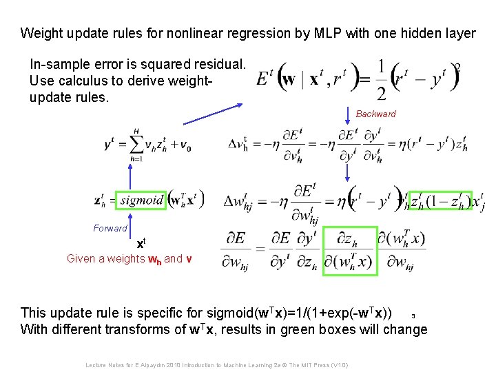
Weight update rules for nonlinear regression by MLP with one hidden layer In-sample error is squared residual. Use calculus to derive weightupdate rules. Backward Forward xt Given a weights wh and v This update rule is specific for sigmoid(w. Tx)=1/(1+exp(-w. Tx)) 3 With different transforms of w. Tx, results in green boxes will change Lecture Notes for E Alpaydın 2010 Introduction to Machine Learning 2 e © The MIT Press (V 1. 0)

Issues in the application of MLPs How many hidden layers? One is sufficient for regression and classification on tabular data. How many nodes in the hidden layer? Minimum is twice the number of output nodes. Can be investigated by a validation set. How many iterations of back propagation for weight refinement? General rule: Stop early to avoid over fitting. Can be investigated by a validation set. How much data is needed? Depends on the number of weights and amount of noise.

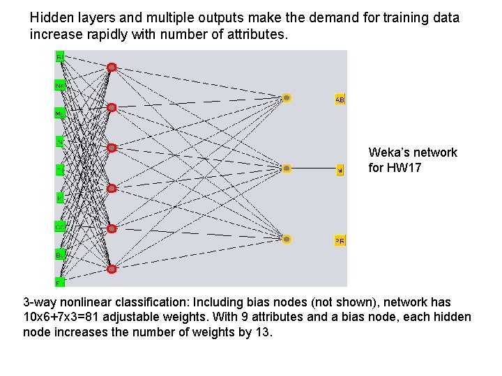
Hidden layers and multiple outputs make the demand for training data increase rapidly with number of attributes. Weka’s network for HW 17 3 -way nonlinear classification: Including bias nodes (not shown), network has 10 x 6+7 x 3=81 adjustable weights. With 9 attributes and a bias node, each hidden node increases the number of weights by 13.

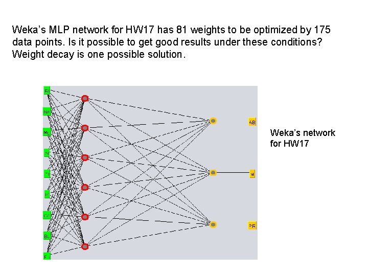
Weka’s MLP network for HW 17 has 81 weights to be optimized by 175 data points. Is it possible to get good results under these conditions? Weight decay is one possible solution. Weka’s network for HW 17

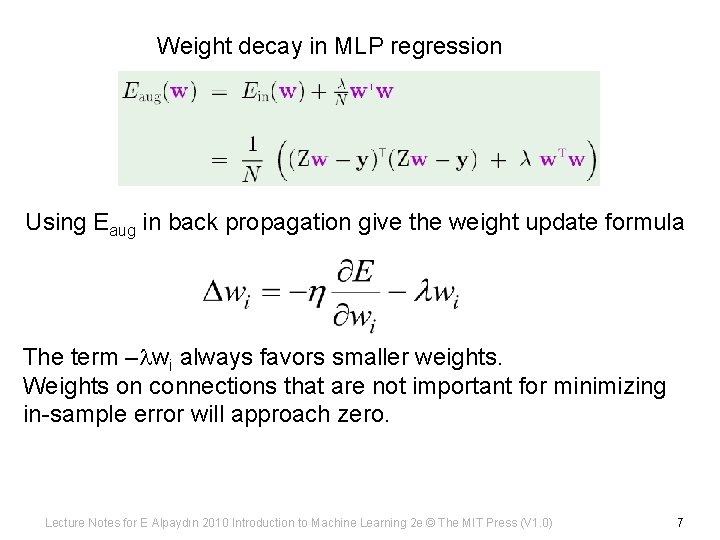
Weight decay in MLP regression Using Eaug in back propagation give the weight update formula The term –lwi always favors smaller weights. Weights on connections that are not important for minimizing in-sample error will approach zero. Lecture Notes for E Alpaydın 2010 Introduction to Machine Learning 2 e © The MIT Press (V 1. 0) 7

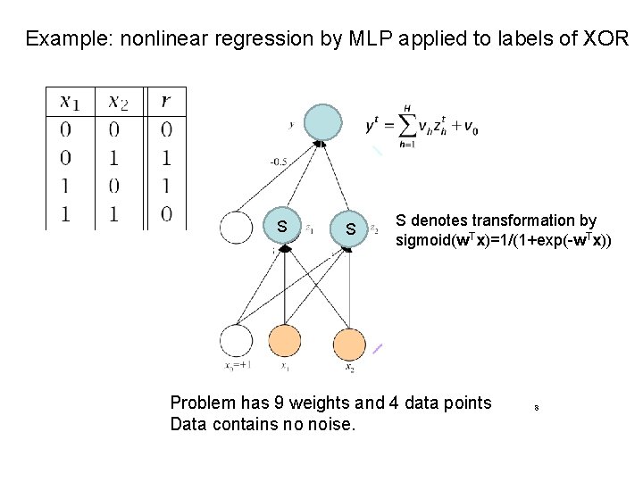
Example: nonlinear regression by MLP applied to labels of XOR S S S denotes transformation by S Tx)=1/(1+exp(-w. Tx)) sigmoid(w Problem has 9 weights and 4 data points Data contains no noise. 8

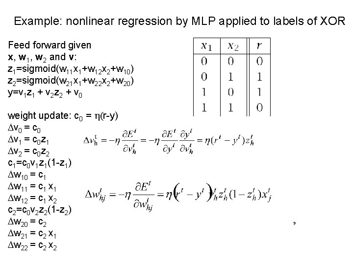
Example: nonlinear regression by MLP applied to labels of XOR Feed forward given x, w 1, w 2 and v: z 1=sigmoid(w 11 x 1+w 12 x 2+w 10) z 2=sigmoid(w 21 x 1+w 22 x 2+w 20) y=v 1 z 1 + v 2 z 2 + v 0 weight update: c 0 = h(r-y) Dv 0 = c 0 Dv 1 = c 0 z 1 Dv 2 = c 0 z 2 c 1=c 0 v 1 z 1(1 -z 1) Dw 10 = c 1 Dw 11 = c 1 x 1 Dw 12 = c 1 x 2 c 2=c 0 v 2 z 2(1 -z 2) Dw 20 = c 2 Dw 21 = c 2 x 1 Dw 22 = c 2 x 2 9

Perform 1000 iterations with the example chosen randomly from the dataset. Before each weight update, calculate the sum of squared residuals and save for a plot of convergence. With the final weights, calculate the values z 1, z 2 and y for each example in the dataset.

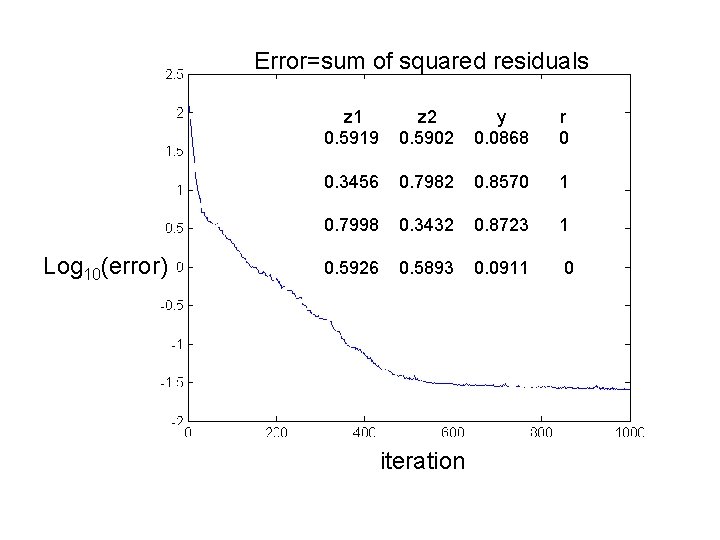
Error=sum of squared residuals Log 10(error) z 1 0. 5919 z 2 0. 5902 y 0. 0868 r 0 0. 3456 0. 7982 0. 8570 1 0. 7998 0. 3432 0. 8723 1 0. 5926 0. 5893 0. 0911 0 iteration

General application of a validation set to find the best model complexity As “complexity” increases (e. g. , more attributes, higher degree of polynomial, etc. ) expect a better fit (smaller in-sample error). Small in-sample error is not the only important aspect of a good model. “Generalization” is how well the model performs on examples not in the training set. “Over fitting” means decreasing in-sample error to the point that generalization is compromised. A “validation set” lets us find the best trade-off between insample error and generalization.

Example from polynomial regression: Generate the in silico data set of 2 sin(1. 5 x)+N(0, 1) with 100 uniformly distributed random values of x between 0 and 5 and 100 normally distributed values of noise with zero mean and unit variance. Divide data into training and validation sets. Fit polynomials of degree 1 – 5 to the training set. For each case use the model with minimum in-sample error to calculate the error in application to the validation set. Plot Ein and Eval vs degree of polynomial. Use the plot to decide the best degree of polynomial

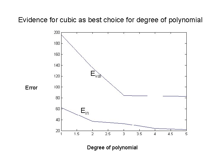
Evidence for cubic as best choice for degree of polynomial Eval Error Ein Degree of polynomial

Applications of validation set to MLPs In polynomial regression the validation subset can be returned to training set after the best degree has been determined. Not true with MLP non-linear regression. With MLP, we cannot expect the results revealed by a validation set to hold if back propagation is repeated with new training set that is old training set + validation set. With MLP back propagation, Eval is more like Etest, examples never used in training.

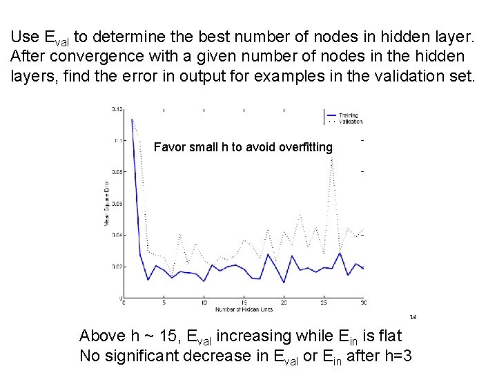
Use Eval to determine the best number of nodes in hidden layer. After convergence with a given number of nodes in the hidden layers, find the error in output for examples in the validation set. Favor small h to avoid overfitting 16 Above h ~ 15, Eval increasing while Ein is flat No significant decrease in Eval or Ein after h=3

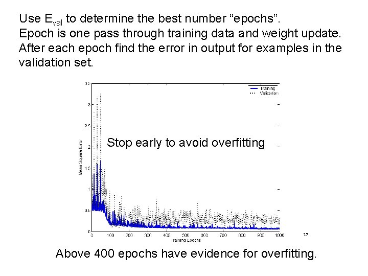
Use Eval to determine the best number “epochs”. Epoch is one pass through training data and weight update. After each epoch find the error in output for examples in the validation set. Stop early to avoid overfitting 17 Above 400 epochs have evidence for overfitting.

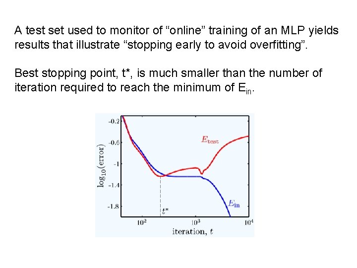
A test set used to monitor of “online” training of an MLP yields results that illustrate “stopping early to avoid overfitting”. Best stopping point, t*, is much smaller than the number of iteration required to reach the minimum of Ein.

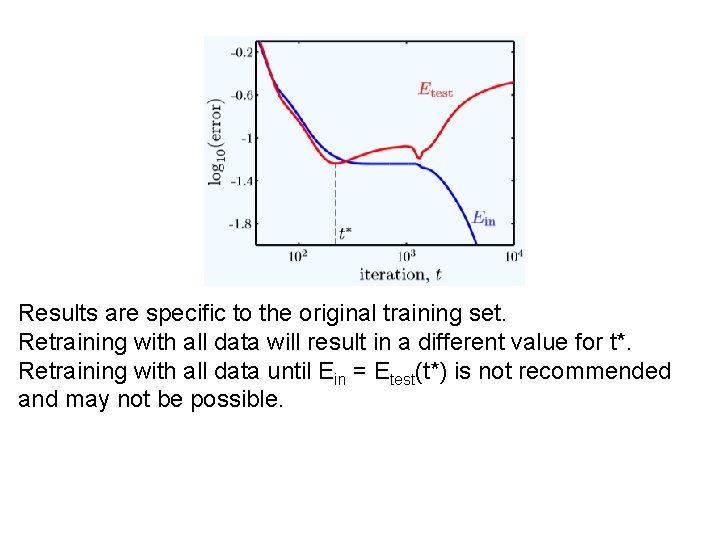
Results are specific to the original training set. Retraining with all data will result in a different value for t*. Retraining with all data until Ein = Etest(t*) is not recommended and may not be possible.

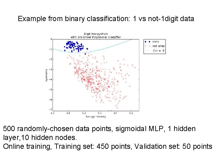
Example from binary classification: 1 vs not-1 digit data 500 randomly-chosen data points, sigmoidal MLP, 1 hidden layer, 10 hidden nodes. Online training, Training set: 450 points, Validation set: 50 points

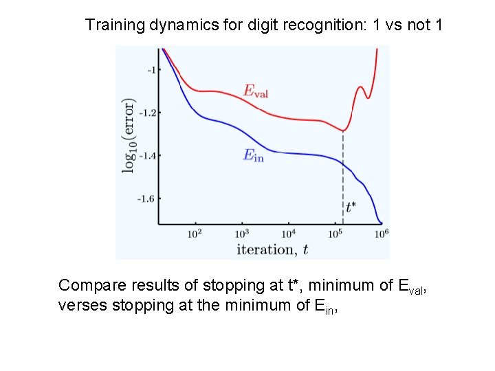
Training dynamics for digit recognition: 1 vs not 1 Compare results of stopping at t*, minimum of Eval, verses stopping at the minimum of Ein,

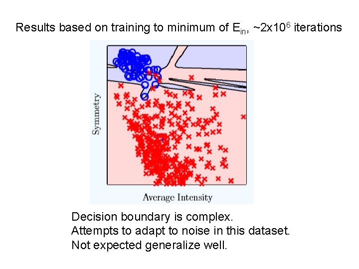
Results based on training to minimum of Ein, ~2 x 106 iterations Decision boundary is complex. Attempts to adapt to noise in this dataset. Not expected generalize well.

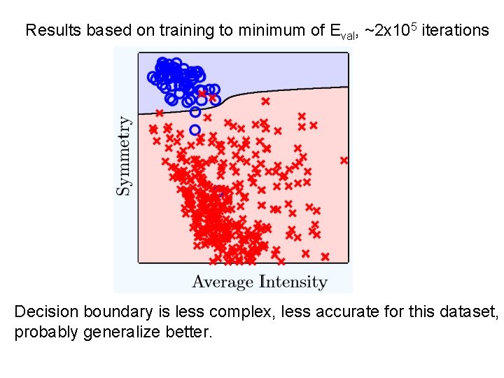
Results based on training to minimum of Eval, ~2 x 105 iterations Decision boundary is less complex, less accurate for this dataset, probably generalize better.