VLSI Physical Design Automation Lecture 4 Circuit Partitioning

VLSI Physical Design Automation Lecture 4. Circuit Partitioning (II) Prof. David Pan dpan@ece. utexas. edu Office: ACES 5. 434 11/10/2020 1

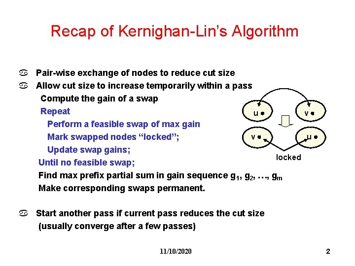
Recap of Kernighan-Lin’s Algorithm a Pair-wise exchange of nodes to reduce cut size a Allow cut size to increase temporarily within a pass Compute the gain of a swap Repeat u v Perform a feasible swap of max gain v u Mark swapped nodes “locked”; Update swap gains; locked Until no feasible swap; Find max prefix partial sum in gain sequence g 1, g 2, …, gm Make corresponding swaps permanent. a Start another pass if current pass reduces the cut size (usually converge after a few passes) 11/10/2020 2

Fiduccia-Mattheyses Algorithm “A Linear-time Heuristics for Improving Network Partitions” 19 th DAC, pages 175 -181, 1982. 11/10/2020 3

Features of FM Algorithm • Modification of KL Algorithm: – – Can handle non-uniform vertex weights (areas) Allow unbalanced partitions Extended to handle hypergraphs Clever way to select vertices to move, run much faster. 11/10/2020 4

Problem Formulation • Input: A hypergraph with – – – Set vertices V. (|V| = n) Set of hyperedges E. (total # pins in netlist = p) Area au for each vertex u in V. Cost ce for each hyperedge in e. An area ratio r. • Output: 2 partitions X & Y such that – Total cost of hyperedges cut is minimized. – area(X) / (area(X) + area(Y)) is about r. • This problem is NP-Complete!!! 11/10/2020 5

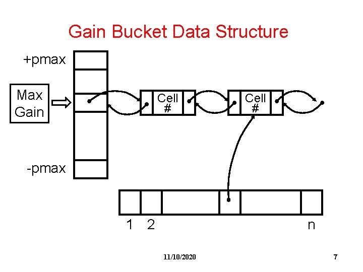
Ideas of FM Algorithm • Similar to KL: – Work in passes. – Lock vertices after moved. – Actually, only move those vertices up to the maximum partial sum of gain. • Difference from KL: – Not exchanging pairs of vertices. Move only one vertex at each time. – The use of gain bucket data structure. 11/10/2020 6

Gain Bucket Data Structure +pmax Max Gain Cell # -pmax 1 2 n 11/10/2020 7

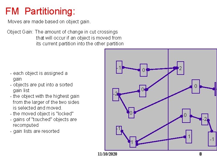
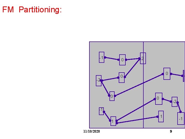
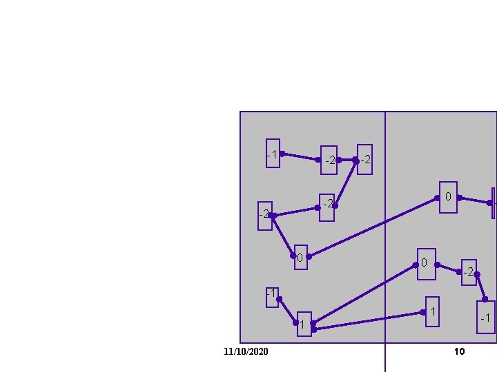
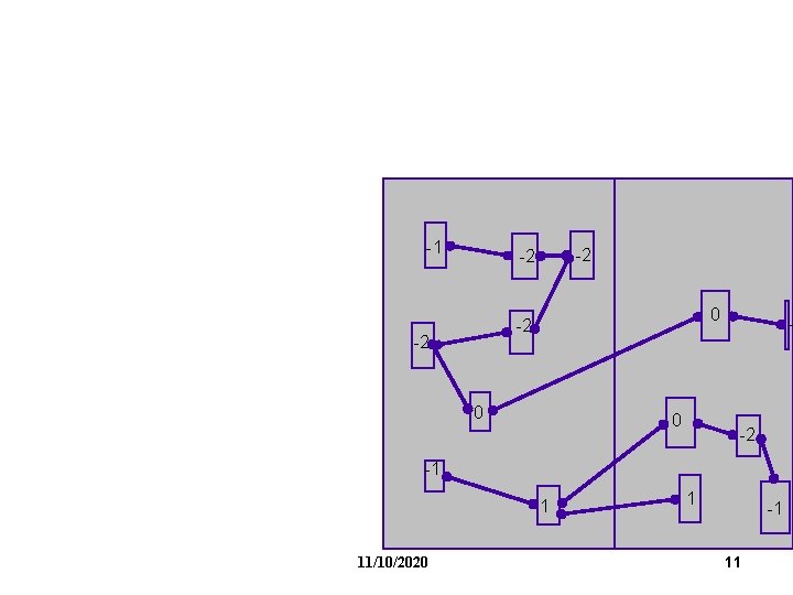
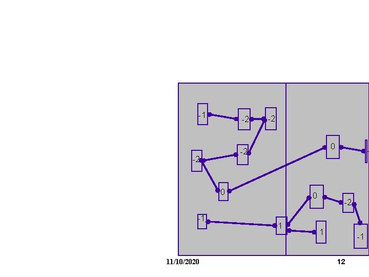
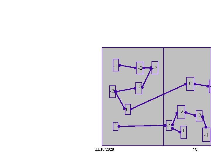
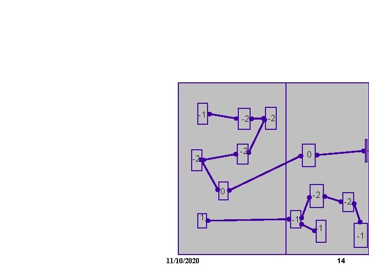
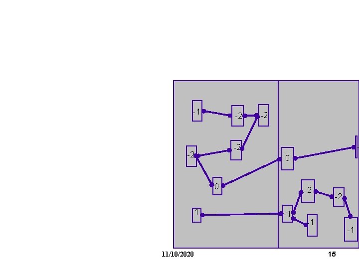
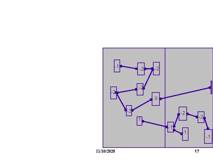
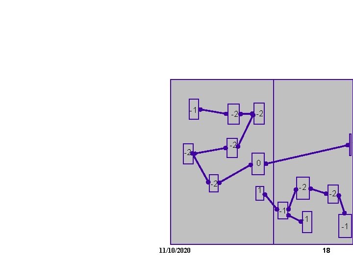
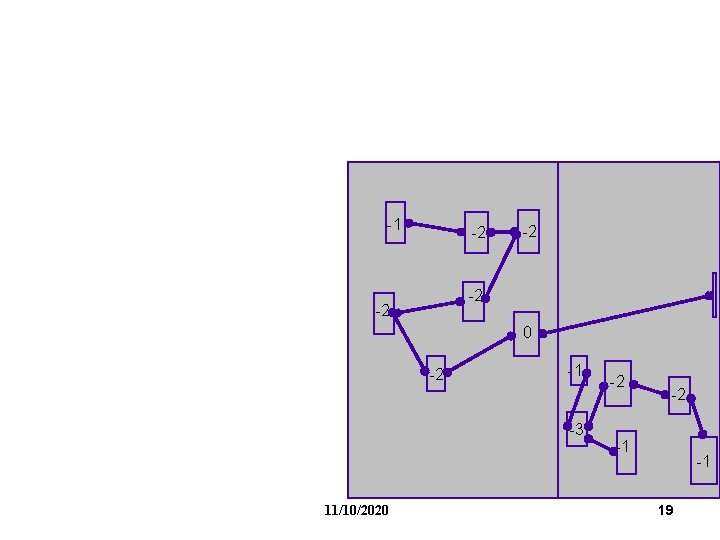
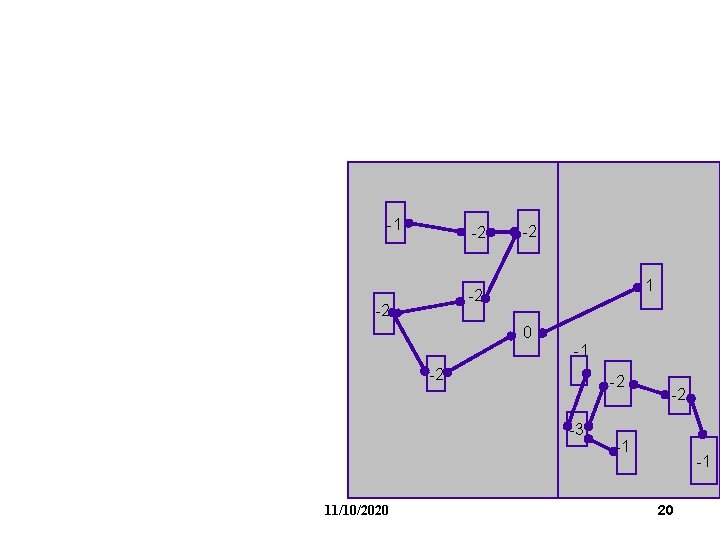
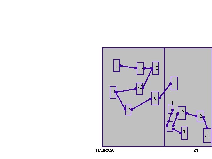
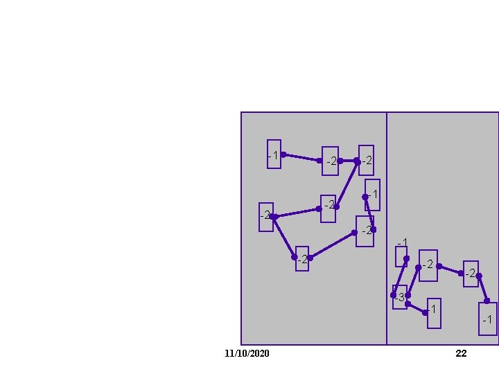
FM Partitioning: Moves are made based on object gain. Object Gain: The amount of change in cut crossings that will occur if an object is moved from its current partition into the other partition - each object is assigned a gain - objects are put into a sorted gain list - the object with the highest gain from the larger of the two sides is selected and moved. - the moved object is "locked" - gains of "touched" objects are recomputed - gain lists are resorted -1 0 2 0 0 -2 -1 1 11/10/2020 8

FM Partitioning: -1 0 2 0 0 -2 -1 1 11/10/2020 9

-1 -2 -2 0 0 - -2 -1 1 11/10/2020 10

-1 -2 -2 0 0 - -2 -1 1 11/10/2020 1 -1 11

-1 -2 -2 0 -1 11/10/2020 0 1 - -2 1 -1 12

-1 -2 -2 0 1 11/10/2020 -2 -1 -1 13

-1 -2 -2 0 1 11/10/2020 - 0 -2 -1 -1 14

-1 -2 -2 -2 0 0 1 11/10/2020 -2 -1 -1 15

-1 -2 -2 0 -2 1 11/10/2020 -2 -1 -1 16

-1 -2 -2 0 -2 -2 1 -1 11/10/2020 -2 -1 -1 17

-1 -2 -2 0 -2 -2 1 -1 11/10/2020 -2 -1 -1 18

-1 -2 -2 0 -2 -1 -3 11/10/2020 -2 -2 -1 -1 19

-1 -2 -2 0 -1 -2 -2 -3 11/10/2020 -2 -1 -1 20

-1 -2 -2 0 -1 -2 -2 -3 11/10/2020 -2 -1 -1 21

-1 -2 -2 -3 11/10/2020 -2 -1 -1 22

Time Complexity of FM • For each pass, – Constant time to find the best vertex to move. – After each move, time to update gain buckets is proportional to degree of vertex moved. – Total time is O(p), where p is total number of pins • Number of passes is usually small. 11/10/2020 23

Extension by Krishnamurthy “An Improved Min-Cut Algorithm for Partitioning VLSI Networks”, IEEE Trans. Computer, 33(5): 438 -446, 1984. 11/10/2020 24

Tie-Breaking Strategy • For each vertex, instead of having a gain bucket, a gain vector is used. • Gain vector is a sequence of potential gain values corresponding to numbers of possible moves into the future. • Therefore, rth entry looks r moves ahead. • Time complexity is O(pr), where r is max # of lookahead moves stored in gain vector. • If ties still occur, some researchers observe that LIFO order improves solution quality. 11/10/2020 25

Ratio Cut Objective by Wei and Cheng “Towards Efficient Hierarchical Designs by Ratio Cut Partitioning”, ICCAD, pages 1: 298 -301, 1989. 11/10/2020 26

Ratio Cut Objective • It is not desirable to have some pre-defined ratio on the partition sizes. • Wei and Cheng proposed the Ratio Cut objective. • Try to locate natural clusters in circuit and force the partitions to be of similar sizes at the same time. • Ratio Cut RXY = CXY/(|X| x |Y|) • A heuristic based on FM was proposed. 11/10/2020 27

Sanchis Algorithm “Multiple-way Network Partitioning”, IEEE Trans. Computers, 38(1): 62 -81, 1989. 11/10/2020 28

Multi-Way Partitioning • Dividing into more than 2 partitions. • Algorithm by extending the idea of FM + Krishnamurthy. 11/10/2020 29

Partitioning: Simulated Annealing 11/10/2020 30

State Space Search Problem • Combinatorial optimization problems (like partitioning) can be thought as a State Space Search Problem. • A State is just a configuration of the combinatorial objects involved. • The State Space is the set of all possible states (configurations). • A Neighbourhood Structure is also defined (which states can one go in one step). • There is a cost corresponding to each state. • Search for the min (or max) cost state. 11/10/2020 31

Greedy Algorithm • A very simple technique for State Space Search Problem. • Start from any state. • Always move to a neighbor with the min cost (assume minimization problem). • Stop when all neighbors have a higher cost than the current state. 11/10/2020 32

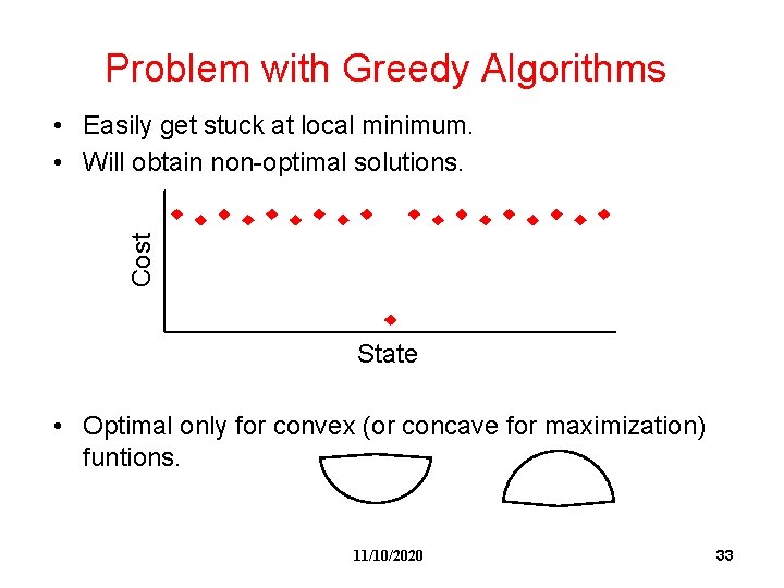
Problem with Greedy Algorithms Cost • Easily get stuck at local minimum. • Will obtain non-optimal solutions. State • Optimal only for convex (or concave for maximization) funtions. 11/10/2020 33

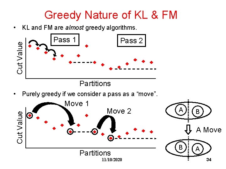
Greedy Nature of KL & FM Cut Value • KL and FM are almost greedy algorithms. Pass 1 Pass 2 Partitions • Purely greedy if we consider a pass as a “move”. Cut Value Move 1 Move 2 A B A Move Partitions 11/10/2020 B A 34

Simulated Annealing • Very general search technique. • Try to avoid being trapped in local minimum by making probabilistic moves. • Popularize as a heuristic for optimization by: – Kirkpatrick, Gelatt and Vecchi, “Optimization by Simulated Annealing”, Science, 220(4598): 498 -516, May 1983. 11/10/2020 35

Basic Idea of Simulated Annealing • Inspired by the Annealing Process: – The process of carefully cooling molten metals in order to obtain a good crystal structure. – First, metal is heated to a very high temperature. – Then slowly cooled. – By cooling at a proper rate, atoms will have an increased chance to regain proper crystal structure. • Attaining a min cost state in simulated annealing is analogous to attaining a good crystal structure in annealing. 11/10/2020 36

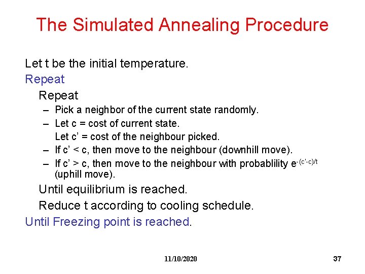
The Simulated Annealing Procedure Let t be the initial temperature. Repeat – Pick a neighbor of the current state randomly. – Let c = cost of current state. Let c’ = cost of the neighbour picked. – If c’ < c, then move to the neighbour (downhill move). – If c’ > c, then move to the neighbour with probablility e-(c’-c)/t (uphill move). Until equilibrium is reached. Reduce t according to cooling schedule. Until Freezing point is reached. 11/10/2020 37

Things to decide when using SA • When solving a combinatorial problem, we have to decide: – – – – The state space The neighborhood structure The cost function The initial state The initial temperature The cooling schedule (how to change t) The freezing point 11/10/2020 38

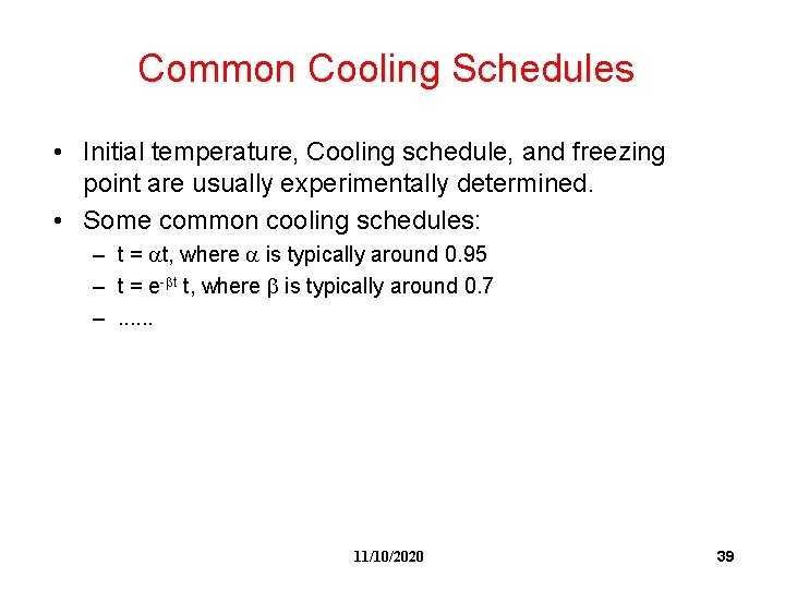
Common Cooling Schedules • Initial temperature, Cooling schedule, and freezing point are usually experimentally determined. • Some common cooling schedules: – t = at, where a is typically around 0. 95 – t = e-bt t, where b is typically around 0. 7 –. . . 11/10/2020 39

Paper by Johnson, Aragon, Mc. Geoch and Schevon on Bisectioning using SA “Optimization by Simulated Annealing: An Experimental Evaluation Part I, Graph Partitioning”, Operations Research, 37: 865 -892, 1989. 11/10/2020 40

The Work of Johnson, et al. • An extensive empirical study of Simulated Annealing versus Iterative Improvement Approaches. • Conclusion: SA is a competitive approach, getting better solutions than KL for random graphs. Remarks: – Netlists are not random graphs, but sparse graphs with local structure. – SA is too slow. So KL/FM variants are still most popular. – Multiple runs of KL/FM variants with random initial solutions may be preferable to SA. 11/10/2020 41

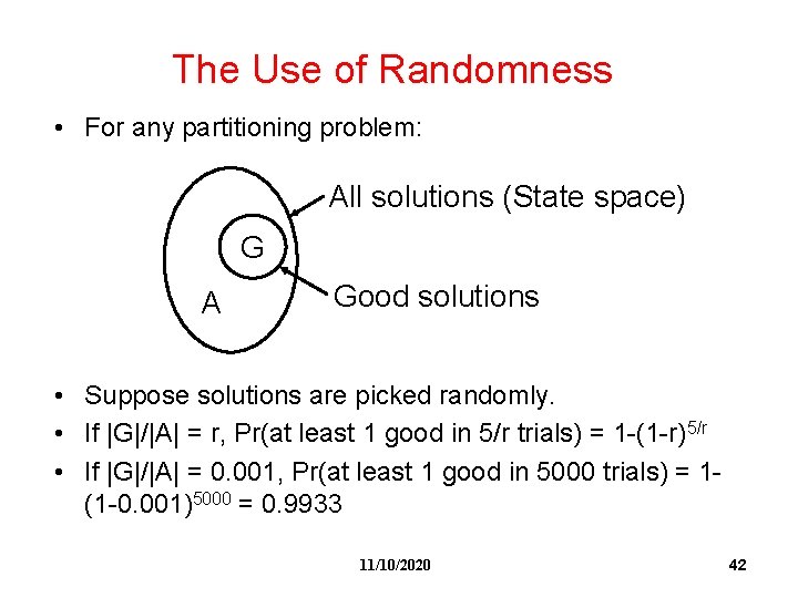
The Use of Randomness • For any partitioning problem: All solutions (State space) G A Good solutions • Suppose solutions are picked randomly. • If |G|/|A| = r, Pr(at least 1 good in 5/r trials) = 1 -(1 -r)5/r • If |G|/|A| = 0. 001, Pr(at least 1 good in 5000 trials) = 1(1 -0. 001)5000 = 0. 9933 11/10/2020 42

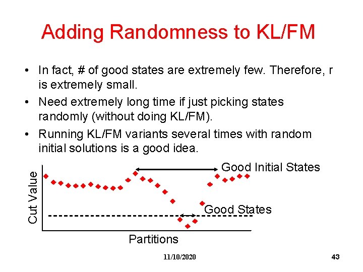
Adding Randomness to KL/FM • In fact, # of good states are extremely few. Therefore, r is extremely small. • Need extremely long time if just picking states randomly (without doing KL/FM). • Running KL/FM variants several times with random initial solutions is a good idea. Cut Value Good Initial States Good States Partitions 11/10/2020 43

Some Other Approaches • KL/FM-SA Hybrid: Use KL/FM variant to find a good initial solution for SA, then improve that solution by SA at low temperature. • Tabu Search • Genetic Algorithm • Spectral Methods (finding Eigenvectors) • Network Flows • Quadratic Programming • . . . 11/10/2020 44

Partitioning: Multi-Level Technique 11/10/2020 45

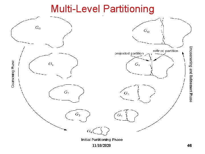
Multi-Level Partitioning 11/10/2020 46

Multilevel Hypergraph Partitioning: Applications in VLSI Domain G. Karypis, R. Aggarwal, V. Kumar and S. Shekhar, DAC 1997. 11/10/2020 47

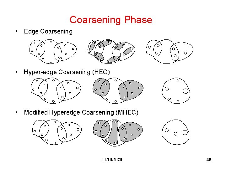
Coarsening Phase • Edge Coarsening • Hyper-edge Coarsening (HEC) • Modified Hyperedge Coarsening (MHEC) 11/10/2020 48

Uncoarsening and Refinement Phase 1. • FM: Based on FM with two simplifications: – – 2. • Limit number of passes to 2 Early-Exit FM (FM-EE), stop each pass if k vertex moves do not improve the cut HER (Hyperedge Refinement) Move a group of vertices between partitions so that an entire hyperedge is removed from the cut 11/10/2020 49

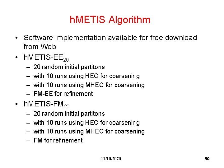
h. METIS Algorithm • Software implementation available for free download from Web • h. METIS-EE 20 – – 20 random initial partitons with 10 runs using HEC for coarsening with 10 runs using MHEC for coarsening FM-EE for refinement • h. METIS-FM 20 – – 20 random initial partitons with 10 runs using HEC for coarsening with 10 runs using MHEC for coarsening FM for refinement 11/10/2020 50

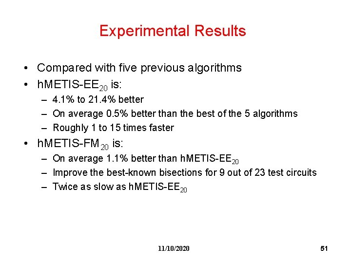
Experimental Results • Compared with five previous algorithms • h. METIS-EE 20 is: – 4. 1% to 21. 4% better – On average 0. 5% better than the best of the 5 algorithms – Roughly 1 to 15 times faster • h. METIS-FM 20 is: – On average 1. 1% better than h. METIS-EE 20 – Improve the best-known bisections for 9 out of 23 test circuits – Twice as slow as h. METIS-EE 20 11/10/2020 51