VLSI Layout Design Methods Layout Design Steps Partitioning

VLSI Layout Design Methods

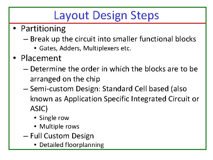
Layout Design Steps • Partitioning – Break up the circuit into smaller functional blocks • Gates, Adders, Multiplexers etc. • Placement – Determine the order in which the blocks are to be arranged on the chip – Semi-custom Design: Standard Cell based (also known as Application Specific Integrated Circuit or ASIC) • Single row • Multiple rows – Full Custom Design • Detailed floorplanning

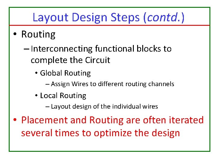
Layout Design Steps (contd. ) • Routing – Interconnecting functional blocks to complete the Circuit • Global Routing – Assign Wires to different routing channels • Local Routing – Layout design of the individual wires • Placement and Routing are often iterated several times to optimize the design

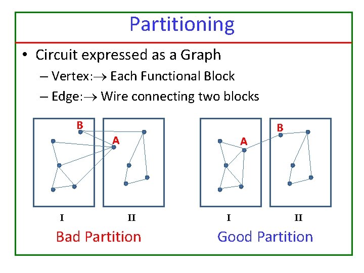
Partitioning • Circuit expressed as a Graph – Vertex: Each Functional Block – Edge: Wire connecting two blocks B A II Bad Partition I B II Good Partition

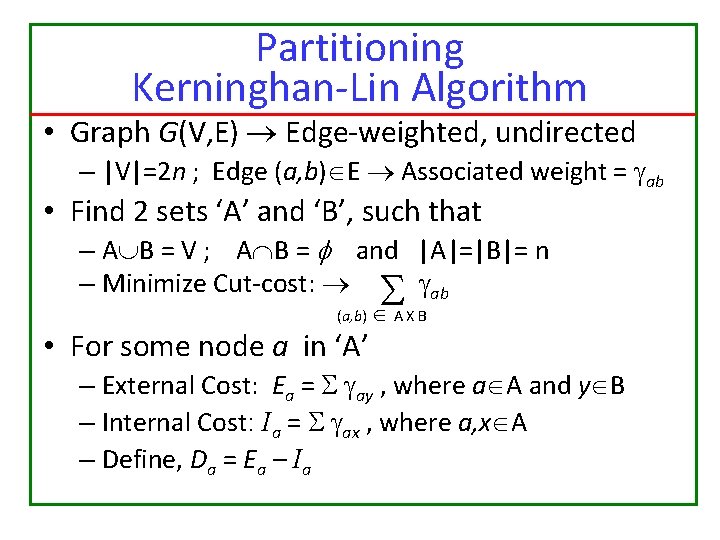
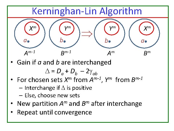
Partitioning Kerninghan-Lin Algorithm • Graph G(V, E) Edge-weighted, undirected – |V|=2 n ; Edge (a, b) E Associated weight = ab • Find 2 sets ‘A’ and ‘B’, such that – A B = V ; A B = and |A|=|B|= n – Minimize Cut-cost: ab (a, b) A X B • For some node a in ‘A’ – External Cost: Ea = ay , where a A and y B – Internal Cost: Ia = ax , where a, x A – Define, Da = Ea – Ia

Kerninghan-Lin Algorithm Xm Ym a b Am-1 Bm-1 Ym b Xm a Am • Gain if a and b are interchanged = Da + Db – 2 ab • For chosen sets Xm from Am-1, Ym from Bm-1 – Interchange if is positive – Else, choose new sets • New partition Am and Bm after interchange • Repeat until convergence Bm

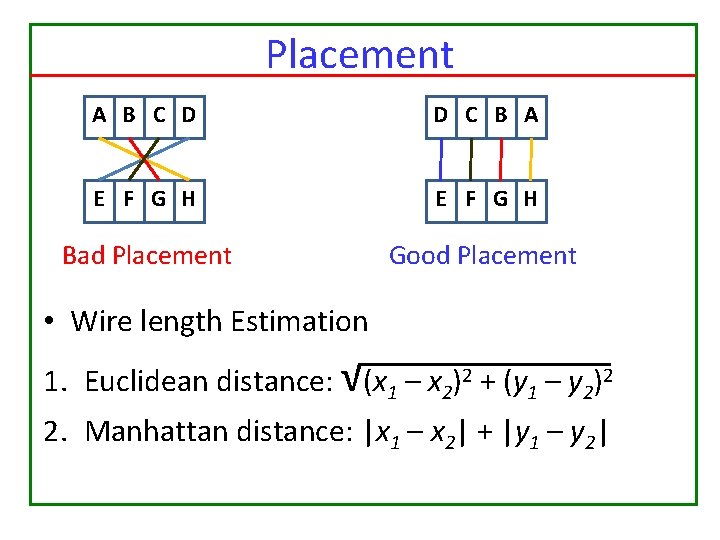
Placement A B C D D C B A E F G H Bad Placement Good Placement • Wire length Estimation 1. Euclidean distance: √(x 1 – x 2)2 + (y 1 – y 2)2 2. Manhattan distance: |x 1 – x 2| + |y 1 – y 2|

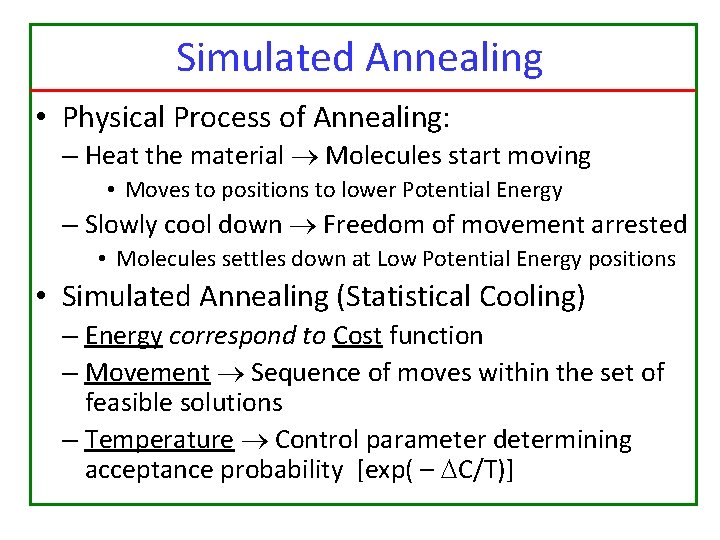
Simulated Annealing • Physical Process of Annealing: – Heat the material Molecules start moving • Moves to positions to lower Potential Energy – Slowly cool down Freedom of movement arrested • Molecules settles down at Low Potential Energy positions • Simulated Annealing (Statistical Cooling) – Energy correspond to Cost function – Movement Sequence of moves within the set of feasible solutions – Temperature Control parameter determining acceptance probability [exp( – C/T)]

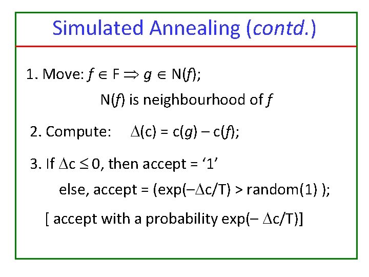
Simulated Annealing (contd. ) 1. Move: f F g N(f); N(f) is neighbourhood of f 2. Compute: (c) = c(g) – c(f); 3. If c 0, then accept = ‘ 1’ else, accept = (exp(– c/T) > random(1) ); [ accept with a probability exp(– c/T)]

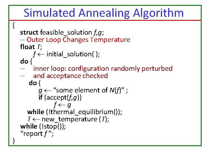
Simulated Annealing Algorithm { } struct feasible_solution f, g; -- Outer Loop Changes Temperature float T; f initial_solution( ); do { -- inner loop: configuration randomly perturbed -- and acceptance checked do { g “some element of N(f)” ; if (accept(f, g)) f g while (!thermal_equilibrium()); T new_temperature (T); while (!stop()); “report f ”;

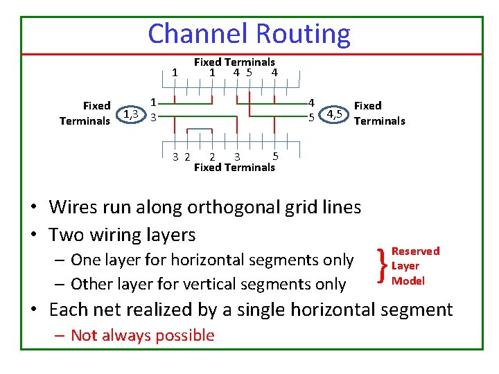
Channel Routing 1 Fixed Terminals 1 4 5 4 1 Floating Fixed 1, 3 3 Terminals 4 Floating Fixed 4, 5 5 Terminals 3 2 5 2 3 Fixed Terminals • Wires run along orthogonal grid lines • Two wiring layers – One layer for horizontal segments only – Other layer for vertical segments only } Reserved Layer Model • Each net realized by a single horizontal segment – Not always possible

Left Edge Algorithm Some Definitions • Interval [xi_min , xi_max] for Net i • Non-overlapping Horizontal segments – Two nets i and j for which xi_max < xj_min – Can be placed on the same row • No. of intervals at any x position : Local density • Max. local density: Channel’s density (d) – Lower bound on channel width Works on problems with no vertical constraint

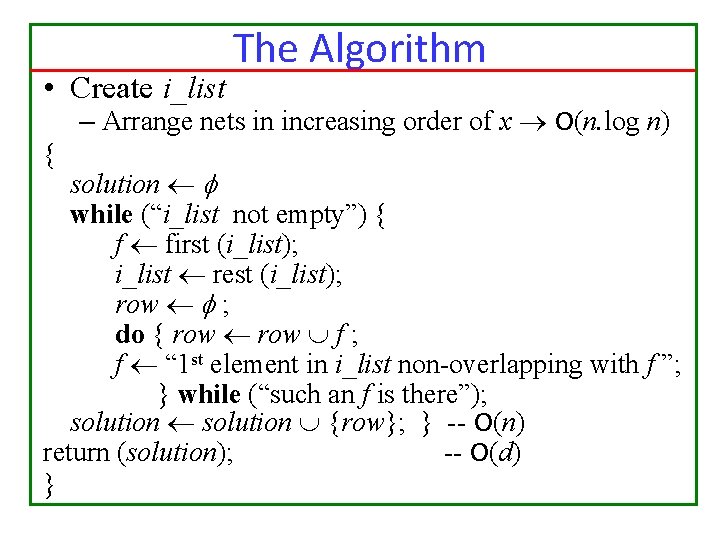
• Create i_list { The Algorithm – Arrange nets in increasing order of x O(n. log n) solution while (“i_list not empty”) { f first (i_list); i_list rest (i_list); row ; do { row f ; f “ 1 st element in i_list non-overlapping with f ”; } while (“such an f is there”); solution {row}; } -- O(n) return (solution); -- O(d) }