Visualizing the Loss Landscape of Neural Nets Team

Visualizing the Loss Landscape of Neural Nets Team Members: Meer Suri, Chandni Akbar, Siffi Singh, Joseph Chataignon, Raphaël Boulanger, Pierric Meunier 1

Outline ❑ Introduction ❑ Loss ❑ and Motivation Function Visualization Technique Effect of Regularization on loss landscape ❑ Effect of depth on the loss landscape ❑ Effect of skip connections on the loss landscape ❑ Visualization ❑ Effect ❑ of the Optimization trajectory of Batch size on the loss landscape Conclusion and References 2

Introduction and Motivation 3

Introduction and Motivation ❑ Ideas taken from the paper “Visualizing the Loss Landscape of Neural Nets” published in NIPS 2018 ❑ To understand the reason behind the common practices and the effects on the underlying loss landscape to know why: ❑ for certain network architecture design (e. g. skip connections) produce loss functions that train easier? ❑ well chosen training parameters (batch size, learning rate, optimizer) produce minimizers that generalize better? ❑ Explore how network architecture affects the loss landscape, and how training parameters affect the shape of minimizers. 4

Loss Function Visualization Technique 5

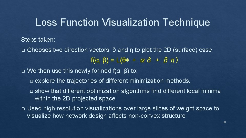
Loss Function Visualization Technique Steps taken: ❑ Chooses two direction vectors, δ and η to plot the 2 D (surface) case f(α, β) = L(θ∗ + αδ + βη) ❑ We then use this newly formed f(α, β) to: ❑ explore the trajectories of different minimization methods. ❑ show that different optimization algorithms find different local minima within the 2 D projected space ❑ Used high-resolution visualizations over large slices of weight space to visualize how network design affects non-convex structure 6

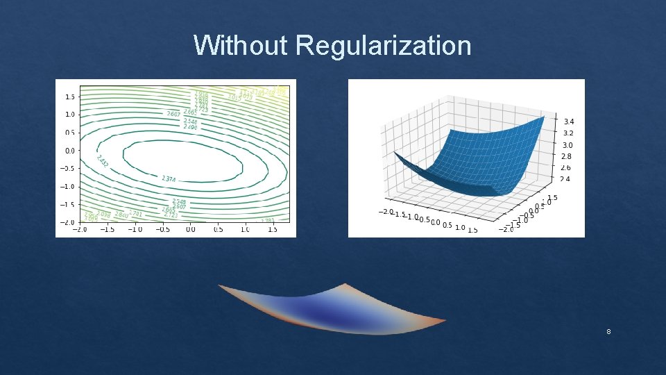
Effect of Regularization on loss landscape 7

Without Regularization 8

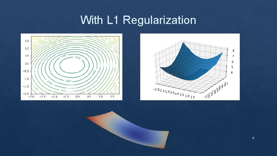
With L 1 Regularization 9

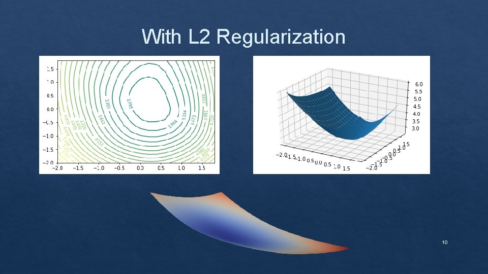
With L 2 Regularization 10

Effect of depth on the loss landscape 11

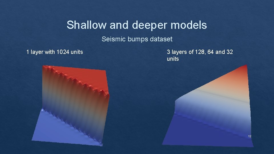
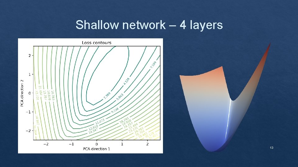
Shallow and deeper models Seismic bumps dataset 1 layer with 1024 units 3 layers of 128, 64 and 32 units 12

Shallow network – 4 layers 13

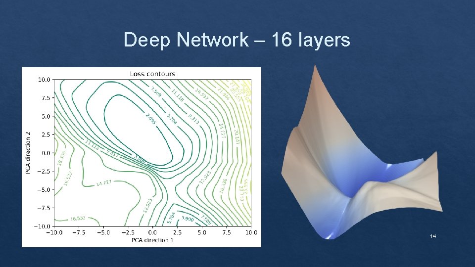
Deep Network – 16 layers 14

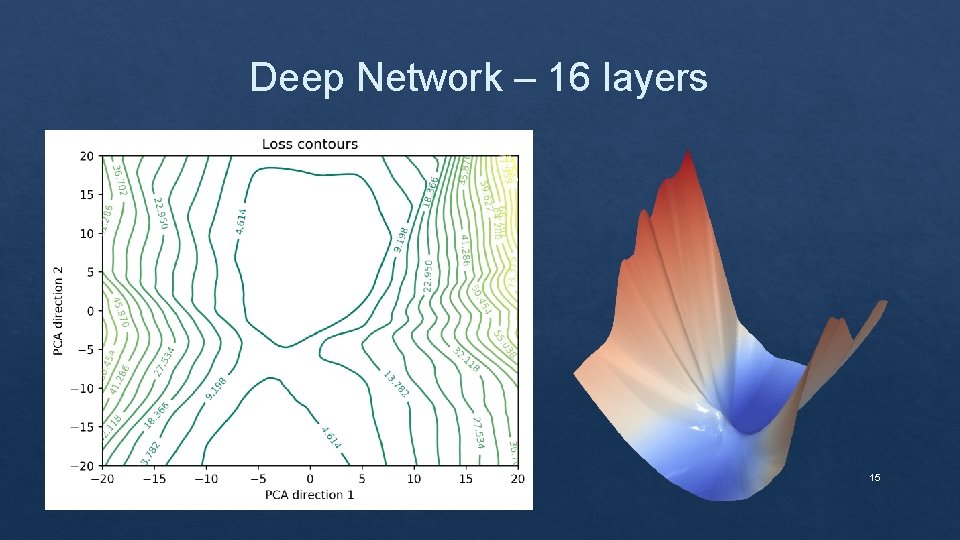
Deep Network – 16 layers 15

Effect of skip connections on the loss landscape 16

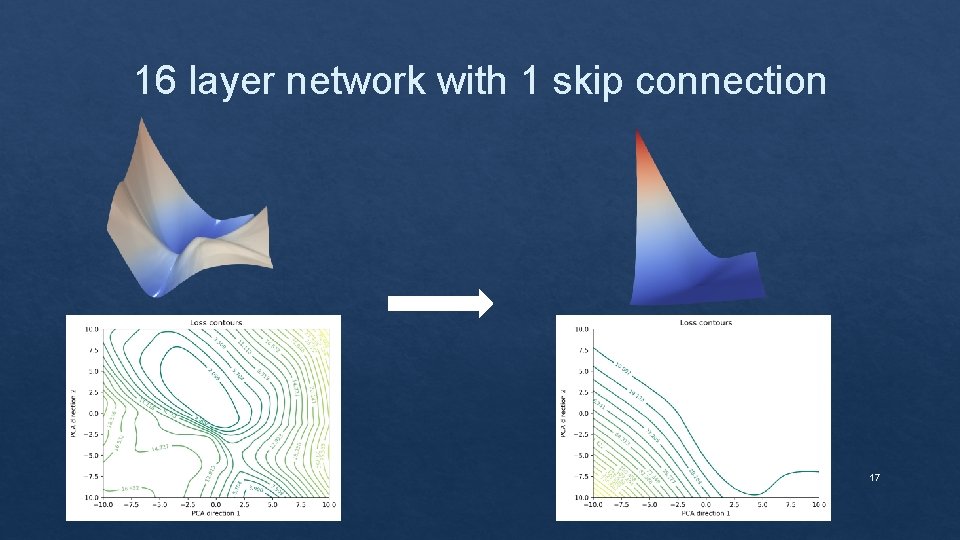
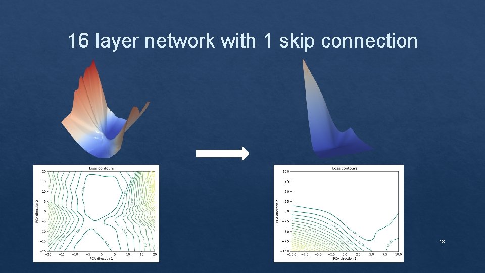
16 layer network with 1 skip connection 17

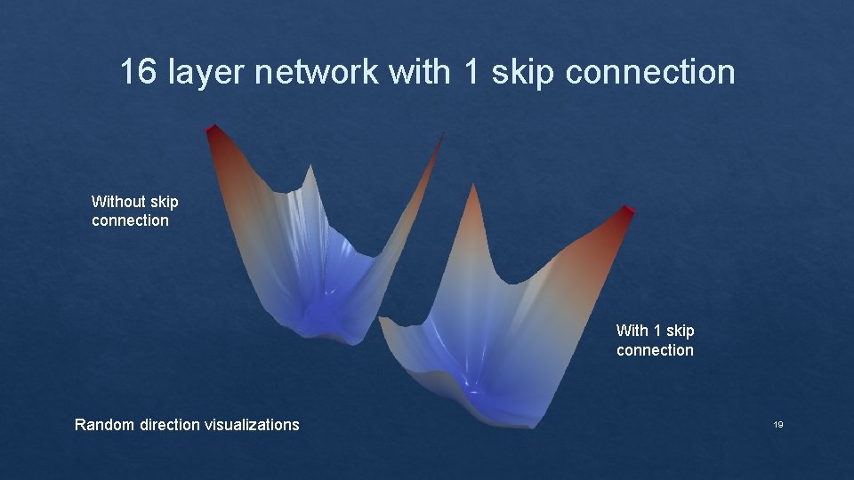
16 layer network with 1 skip connection 18

16 layer network with 1 skip connection Without skip connection With 1 skip connection Random direction visualizations 19

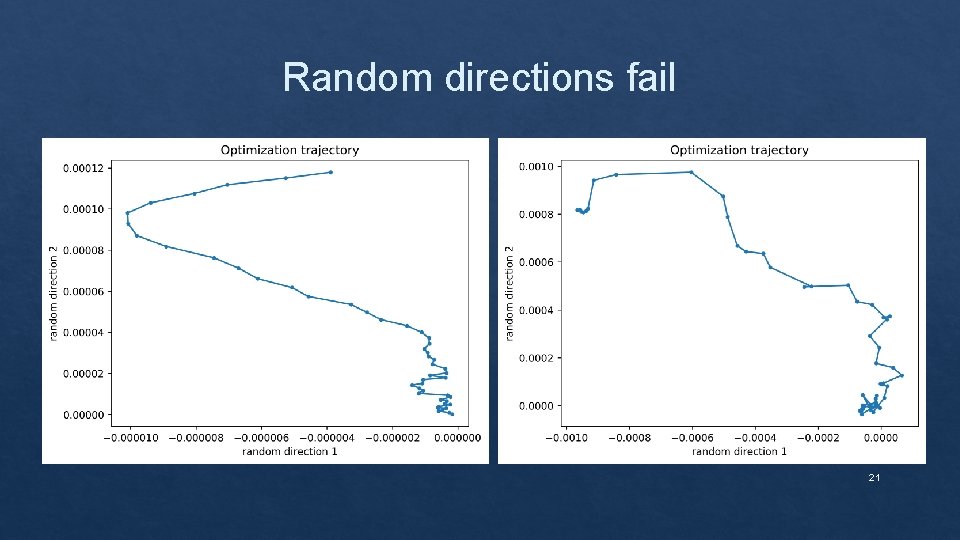
Visualization of the Optimization trajectory 20

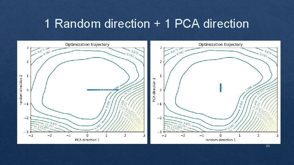
Random directions fail 21

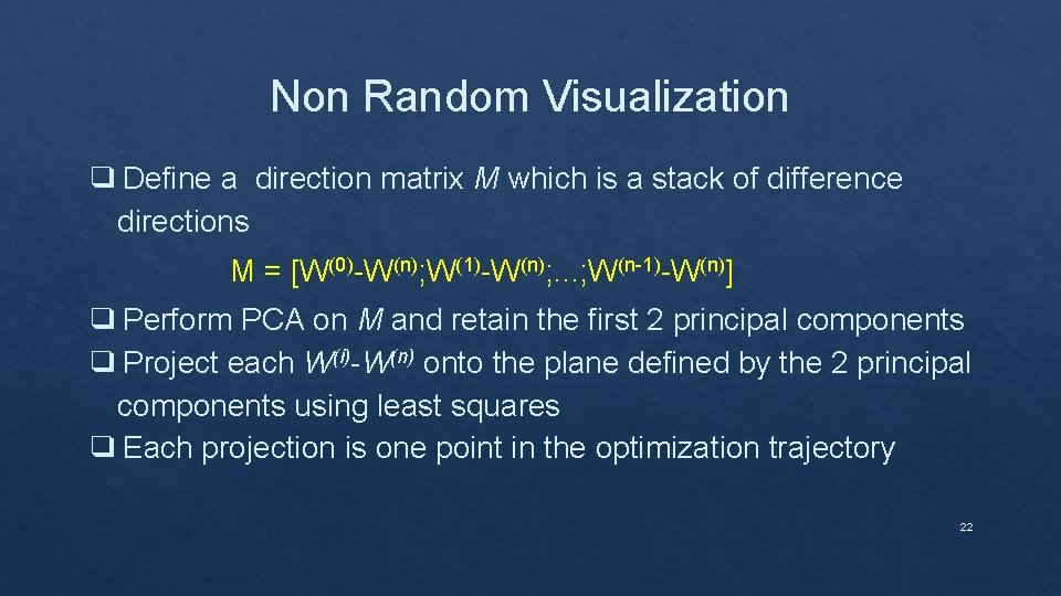
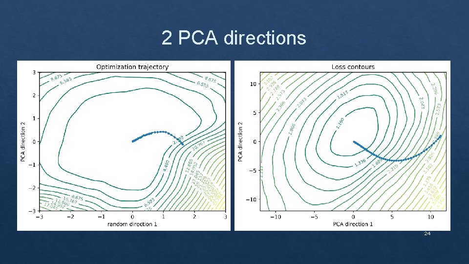
Non Random Visualization ❑ Define a direction matrix M which is a stack of difference directions M = [W(0)-W(n); W(1)-W(n); . . . ; W(n-1)-W(n)] ❑ Perform PCA on M and retain the first 2 principal components ❑ Project each W(i)-W(n) onto the plane defined by the 2 principal components using least squares ❑ Each projection is one point in the optimization trajectory 22

1 Random direction + 1 PCA direction 23

2 PCA directions 24

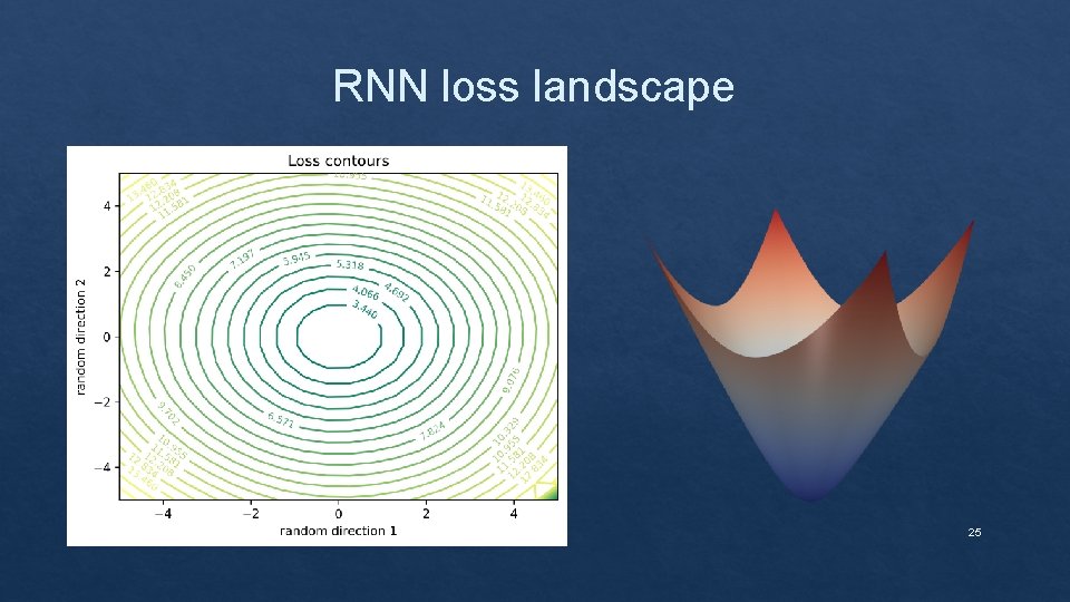
RNN loss landscape 25

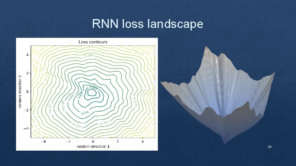
RNN loss landscape 26

Effect of Batch size on the loss landscape 27

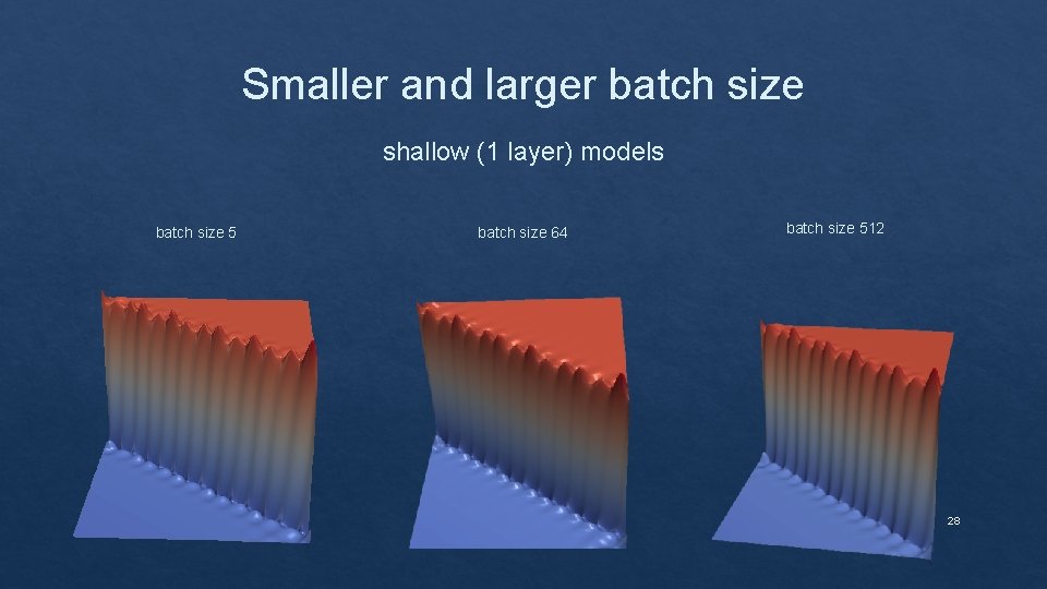
Smaller and larger batch size shallow (1 layer) models batch size 5 batch size 64 batch size 512 28

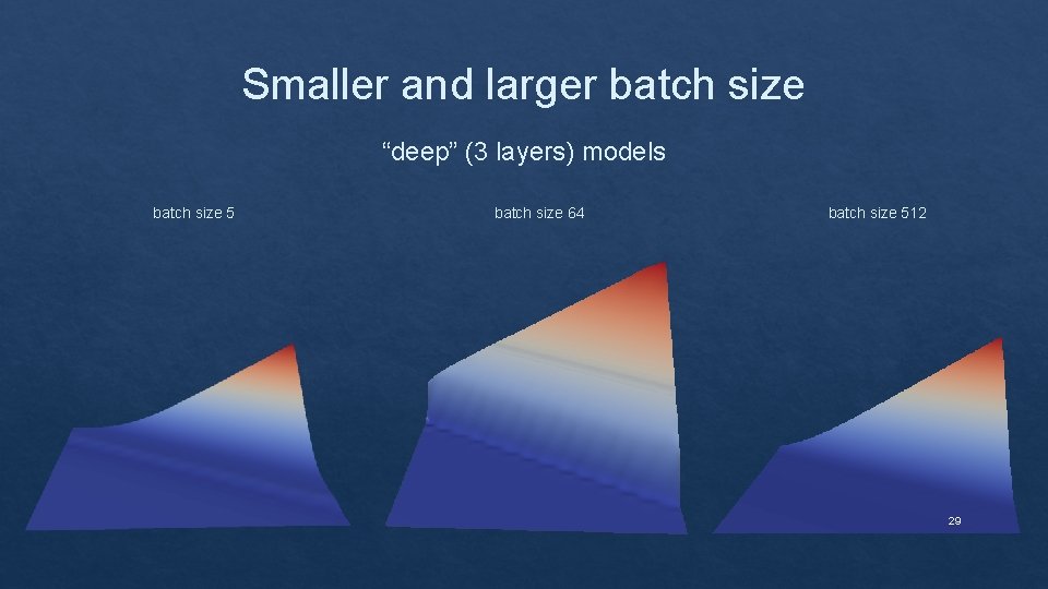
Smaller and larger batch size “deep” (3 layers) models batch size 5 batch size 64 batch size 512 29

Conclusion ❑ Neural networks have advanced dramatically in recent years, largely on anecdotal knowledge and theoretical results with complex assumptions. ❑ A more general understanding of the structure of neural networks is needed, which is why, we tried to provide insights into the consequences of a variety of choices facing the neural network practitioner, including network architecture, regularization, or batch size. ❑ Effective visualization, when coupled with continued advances in theory, should help understanding how the choice of architecture and parameters can influence the optimization of neural networks. 30

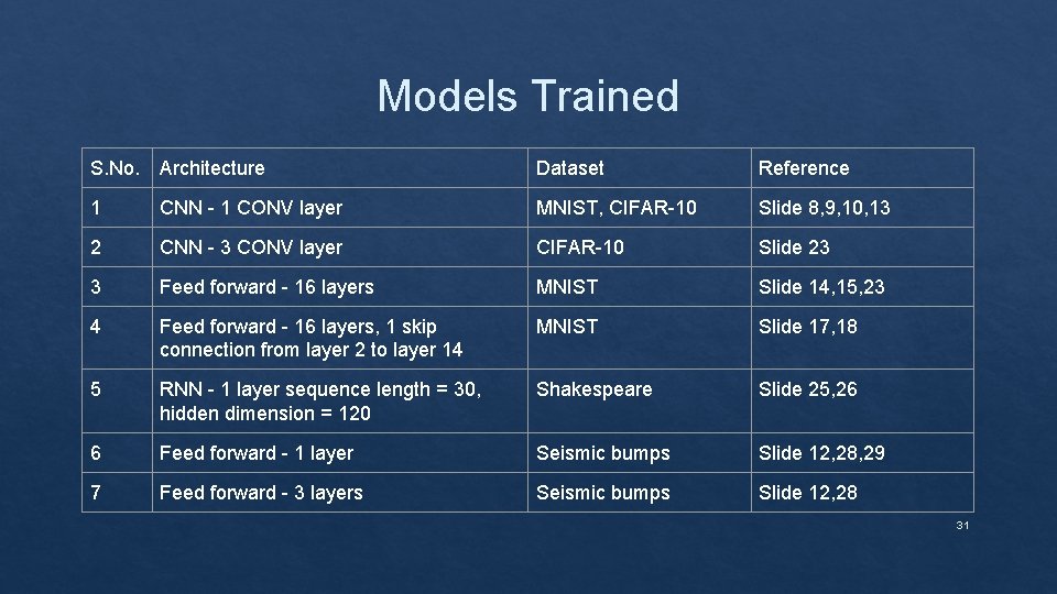
Models Trained S. No. Architecture Dataset Reference 1 CNN - 1 CONV layer MNIST, CIFAR-10 Slide 8, 9, 10, 13 2 CNN - 3 CONV layer CIFAR-10 Slide 23 3 Feed forward - 16 layers MNIST Slide 14, 15, 23 4 Feed forward - 16 layers, 1 skip connection from layer 2 to layer 14 MNIST Slide 17, 18 5 RNN - 1 layer sequence length = 30, hidden dimension = 120 Shakespeare Slide 25, 26 6 Feed forward - 1 layer Seismic bumps Slide 12, 28, 29 7 Feed forward - 3 layers Seismic bumps Slide 12, 28 31

References [1] Paper Link: https: //arxiv. org/pdf/1712. 09913. pdf [2] Git. Hub: https: //github. com/tomgoldstein/loss-landscape [3] Para. View: https: //www. paraview. org/ [4] Visualization of learning in multilayer perceptron networks using principal component analysis. IEEE Transactions on Systems, Man, and Cybernetics. [5] Theory of deep learning ii: Landscape of the empirical risk in deep learning. ar. Xiv preprint ar. Xiv: 1703. 09833, 2017. [6] Seismic-bump dataset: https: //archive. ics. uci. edu/ml/datasets/seismicbumps 32

Thank you for your attention! 33