Visualizing Probabilities Basics of Probability Tools for Visualizing

Visualizing Probabilities Basics of Probability

Tools for Visualizing Probabilities � Contingency � Tree � Tables Diagrams Venn Diagrams

Contingency tables � � � Contingency tables (Two-Way Tables) summarize data about two categorical variables (or factors) collected on the same set of individuals. They can help us visualize and find probabilities of compound events. Each factor can have any number of levels. If the row factor has “r” levels, and the column factor has “c” levels, we say that the two-way table is an “r by c” table.

Two-Way Table Example Suppose High school students were asked whether they smoke and whether their parents smoke � First factor: Parent smoking status ◦ Both parents smoke ◦ One parent smokes ◦ Neither parent smokes � Second factor: Student smoking status ◦ Yes ◦ No So we would have a 3*2 Contingency table here:

Joint probabilities �

Marginal Distributions � We can examine each factor in a two-way table separately by studying the row totals and the column totals. They represent the marginal distributions, expressed in frequencies here

Marginal Distributions cont. . . �

Conditional Distributions � The conditional distribution is the distribution of one factor for each level of the other factor. � Examining data �A these conditional probabilities can show us more about the conditional percent is computed using the counts within a single row or a single column. The denominator is the corresponding row or column total (rather than the table grand total).

Conditional Distributions cont… �

Conditional Distributions cont… �

Simpson’s Paradox � Confounding or lurking variables are always a problem for interpretation, but their impact can be even more drastic when dealing with categorical data. � An association that holds for all of several groups can reverse direction when the data are combined to form a single group. � This reversal is called Simpson's Paradox.

Simpson’s Paradox Example � Consider this table on the failure rates when removing kidney stones in a sample of patients, using one of two procedures: traditional open surgery and a new minimally invasive technique called PCNL. � Does Open surgery PCNL Success 273 289 Failure 77 61 % failure 22 17% the minimally invasive procedure really produce better results than open surgery? What could be going on here?

Simpson’s Paradox Example cont… � The procedures are not chosen randomly by surgeons! � In fact, the minimally invasive procedure is most likely used for smaller stones with a good chance of success, whereas open surgery is more often used for larger stones or more problematic conditions. � When we condition on the size of the stone: Small stones Open surgery PCNL Success 81 234 Failure 6 36 7% 13% % failure Large stones Open surgery PCNL Success 192 55 Failure 71 25 27% 31% % failure

Tree Diagrams �A tree diagram can be helpful to: ◦ Define sample spaces ◦ Picture branching probabilities such as conditionals we want to visualize the sample space for the genders of a 3 child family B B G � Suppose B G G B - BBB G - BBG B - BGB G - BGG B - GBB G - GBG B - GGB G - GGG S = { BBB, BBG, BGB, BGG, GBB, GBG, GGB, GGG } Note: 8 elements, 23

Picturing Events in Venn Diagrams � Compliment ◦ P(A) ◦ P(A’) � Mutually Exclusive: ◦ P(A) ◦ P(B) ◦ Notice A ∩ B does not exist �Symbolically, A ∩ B = Ø � Not Mutually Exclusive: ◦ P(A∩B) ◦ P(A)= P(A∩B’) + P(A∩B) ◦ P(B)= P(B∩A’) + P(A∩B)

Conditional Prob. Example � Surface Flaws Defective Yes(F) No(F') Total Yes(D) 10 18 No(D') 30 342 Total 400 16

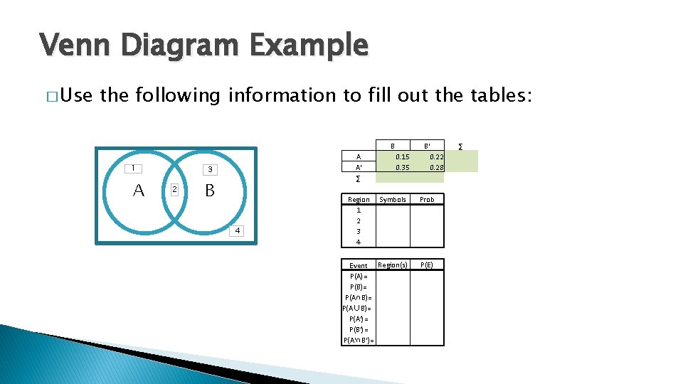
Venn Diagram Example � Use the following information to fill out the tables: B 1 A A A' ∑ 3 2 B 4 B' 0. 22 0. 28 0. 15 0. 35 Region 1 2 3 4 Symbols Prob Event P(A)= P(B)= P(A∩B)= P(A∪B)= P(A')= P(B')= P(A'∩B')= Region(s) P(E) ∑

Venn Diagram Example Solutions � Use the following information to fill out the tables: B 1 A A A' ∑ 3 2 B 4 B' 0. 22 0. 28 0. 15 0. 35 Region 1 2 3 4 Symbols A ∩ B’ A ∩ B A’ ∩ B’ Prob 0. 22 0. 15 0. 35 0. 28 Event P(A)= P(B)= P(A∩B)= P(A∪B)= P(A')= P(B')= P(A'∩B')= Region(s) 1+2 2+3 2 1+2+3 2+3+4 1+2+4 4 P(E) 0. 37 0. 5 0. 15 0. 72 0. 78 0. 65 0. 28 ∑