Visualizing Multivalued Data from 2 D Incompressible Flows

Visualizing Multivalued Data from 2 D Incompressible Flows Using Concepts from Painting R. M. Kirby H. Marmanis D. H. Laidlaw Brown University Presented by Hsin-Ji Wang & Chaoli Wang

l l l l Oil Painting of the Impressionist Basic Fluid Mechanics Concepts Related Work Visualization Methodology Example 1: Rate of Strain Tensor Example 2: Turbulent Charge and Turbulent Current Summary and Conclusions

Oil Painting of the Impressionist l The multiple layers of brush stokes in these paintings provide a natural metaphor of constructing visualization from layers of synthetic “brush stokes”. l The works of three painters they studied – – – Gogh, Vincent van (1853 -1890) Monet, Claude-Oscar (1840 -1926) Cezanne, Paul (1839 -1906)

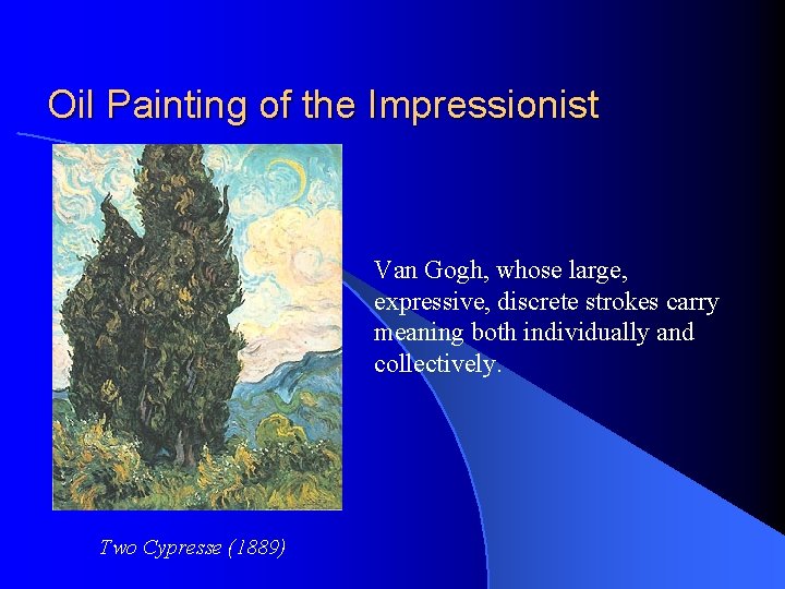
Oil Painting of the Impressionist Van Gogh, whose large, expressive, discrete strokes carry meaning both individually and collectively. Two Cypresse (1889)

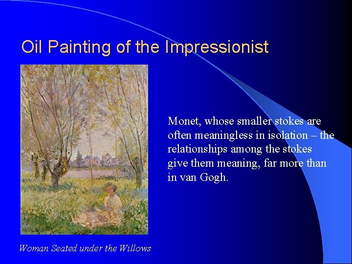
Oil Painting of the Impressionist Monet, whose smaller stokes are often meaningless in isolation – the relationships among the stokes give them meaning, far more than in van Gogh. Woman Seated under the Willows

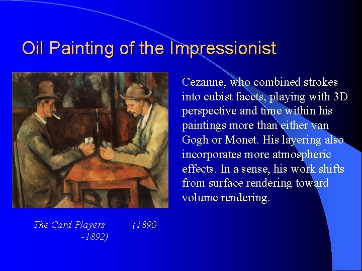
Oil Painting of the Impressionist Cezanne, who combined strokes into cubist facets, playing with 3 D perspective and time within his paintings more than either van Gogh or Monet. His layering also incorporates more atmospheric effects. In a sense, his work shifts from surface rendering toward volume rendering. The Card Players -1892) (1890

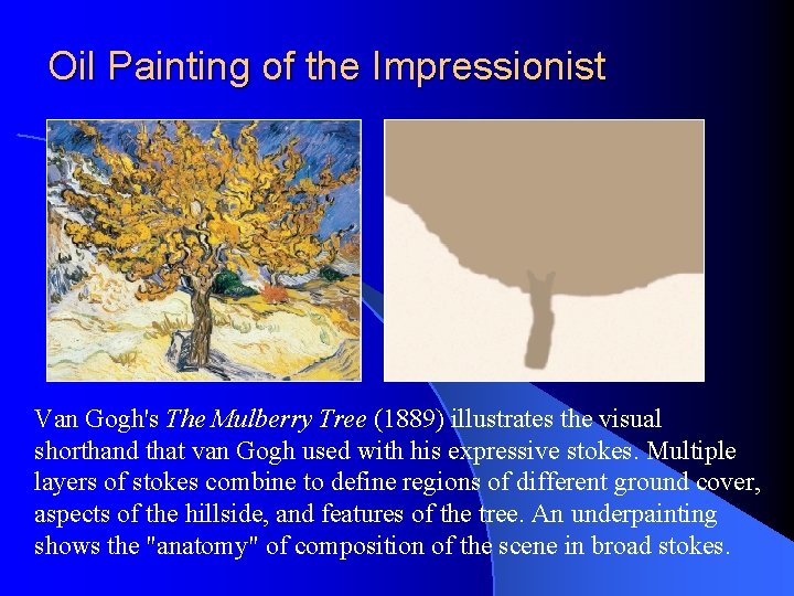
Oil Painting of the Impressionist Van Gogh's The Mulberry Tree (1889) illustrates the visual shorthand that van Gogh used with his expressive stokes. Multiple layers of stokes combine to define regions of different ground cover, aspects of the hillside, and features of the tree. An underpainting shows the "anatomy" of composition of the scene in broad stokes.

Oil Painting of the Impressionist l l Capture the marriage between direct representation of independent data and the overall intuitive feeling of the data as a whole Space: encode different information at different scales Time: design visualizations so that important data features are mapped to quickly seen visual features Choose the artists in whom you have a passionate interest, any artist has lessons to offer to visualization

Basic Fluid Mechanics Concepts l l l Vorticity Reynolds Number Rate of Strain Tensor Turbulent Charge Turbulent Current

Basic Fluid Mechanics Concepts l – – Vorticity ξ=▽×u Vorticity is primarily used to describe the rotation of fluid. If ▽ × u = 0 then the fluid is irrotational else the fluid is rotational

Basic Fluid Mechanics Concepts l – – Reynolds Number Reynolds number = ρVD / μ Reynolds number is proportional to { (inertial force) / (viscous force) } and is used in momentum, heat, and mass transfer to account for dynamic similarity.

Basic Fluid Mechanics Concepts l – – Rate of Strain Tensor The symmetric part is known as the rate of strain tensor The anti-symmetric part is known as vorticity

Basic Fluid Mechanics Concepts l – Turbulent charge and turbulent current The turbulent charge and turbulent current, collectively referred to as turbulent sources, could substitute the role of vorticity in more complicated flows.

Related Work l – – l Multivalued data visualization “Feature-based” methods Statistical methods Icons Layering Flow visualization Spot noise Line integral convolution Computer graphics painting

Visualization Methodology l Developing a visualization method involves – Breaking the data into components Exploring the relationships among components Visually expressing both the components and their relationships – –

Example 1: Rate of Strain Tensor l l – l l l Data breakdown Visualization design Priority Velocity Vorticity Layering Primer Underpainting Ellipse layer Arrow layer Mask layer

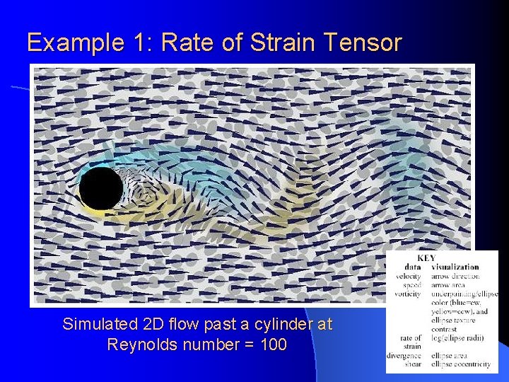
Example 1: Rate of Strain Tensor Simulated 2 D flow past a cylinder at Reynolds number = 100

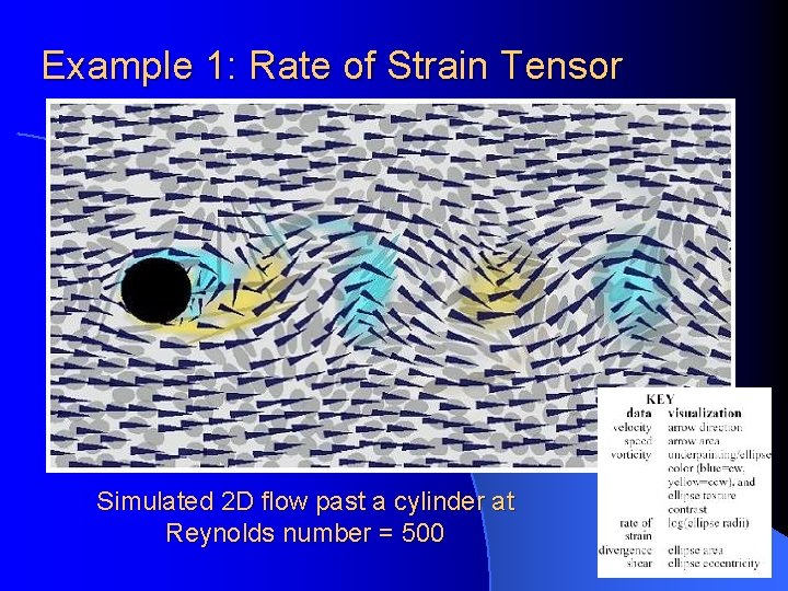
Example 1: Rate of Strain Tensor Simulated 2 D flow past a cylinder at Reynolds number = 500

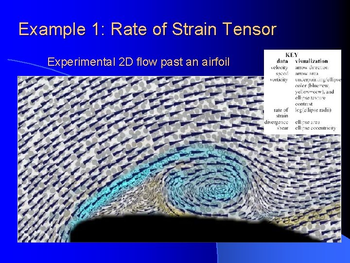
Example 1: Rate of Strain Tensor Experimental 2 D flow past an airfoil

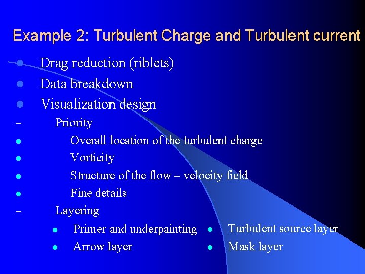
Example 2: Turbulent Charge and Turbulent current l l l – Drag reduction (riblets) Data breakdown Visualization design Priority Overall location of the turbulent charge Vorticity Structure of the flow – velocity field Fine details Layering l l Primer and underpainting Arrow layer l l Turbulent source layer Mask layer

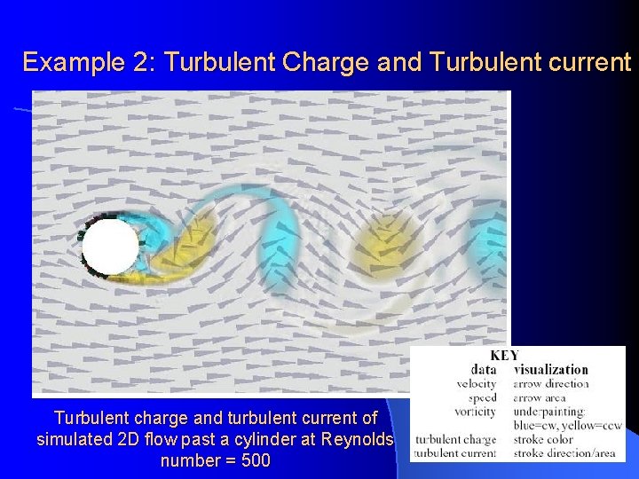
Example 2: Turbulent Charge and Turbulent current Turbulent charge and turbulent current of simulated 2 D flow past a cylinder at Reynolds number = 500

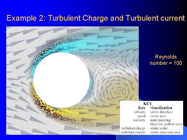
Example 2: Turbulent Charge and Turbulent current Reynolds number = 100

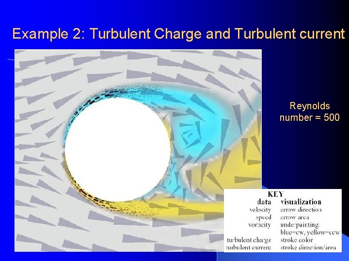
Example 2: Turbulent Charge and Turbulent current Reynolds number = 500

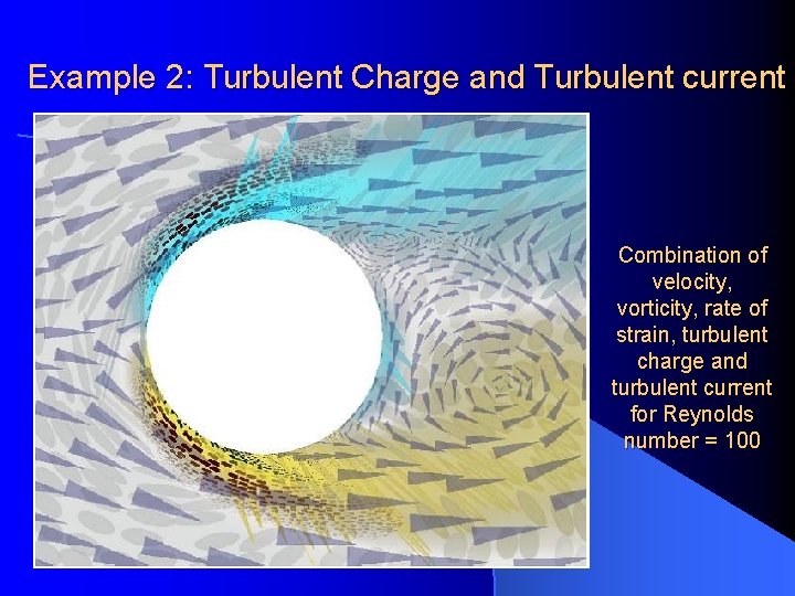
Example 2: Turbulent Charge and Turbulent current Combination of velocity, vorticity, rate of strain, turbulent charge and turbulent current for Reynolds number = 100

Summary and Conclusions l – – – l l l Borrow concepts from oil painting Underpainting Brush strokes Layering Represent many values at each spatial location in different perspectives Get a complete idea of both the dynamics and kinematics of the flow Provide catalyst for future understanding of more complex fluid phenomena

Thank you!